Phonetic Distance Between Words with Application to the International Spelling Alphabet

Introduction

The need to convey letters of an alphabet verbally is a common occurrence. You are on the phone and need to spell a name, car registration number or email address. If you are an English speaker, you will probably be struggling with phases like “‘d’ for ‘dog'” or “‘f’ for ‘Fred'”.

You may just choose to sound the letters directly as ‘de’, ‘ef’, etc. and hope they will be received correctly. With today’s modern, and generally high quality, voice networks this strategy is often successful but occasionally there are misheard letters and you are back to finding a word that represents them or repeating them more slowing and distinctly.

The problem occurs in all languages but this blog will focus on English. However, the principles should be easily transferred to other languages.

How to reliably transmit data over a noisy channel is a well known and much studied problem. The general approach is to include additional information with the original data. This additional or redundant information is used to recover the original data should it be affected during transmission. The trade-off is this additional information makes the transmission longer. So the challenge is to formulate this additional information in a ways that keep the transmission as short as possible but provides the best chance to recover the data should it become corrupted. In the digital domain this comes under the study of Coding Theory.

For our purposes, the additional data is in the form of a word which is used to represent a letter. A word is longer and has more sounds which makes it much easier to identify and less likely to be confused over a noisy background. The words chosen need to be:

  1. Known by the speaker and recipient
  2. Clearly associated with a letter either by agreement or implication
  3. Sufficiently distinct from each another to improve differentiation and recognition
  4. No longer than necessary for expediency

The first for these is accommodated by using well known common words, the second by treating the first letter of the word as the representative letter and the last two are the main design challenge.

Obviously using say, “pat” for “p” and “bat” for “b” is not particularly effective as “pat” and “bat” might themselves be confused. Whereas, for example, “pen” and “bat” seem to be more distinct.

Using long words would make the distinction even greater, for example, “banana” and “pendulum”, however these take longer to say and hence slow down the transmission process. So there is a trade-off between speed and accuracy.

We can summarise the goals of an effective International Spelling Alphabet (or word replacement scheme for letters) as:

  1. Use common words easily recognised by both parties
  2. Use short words to speed communications
  3. Use words that are phonetically distinct to minimise confusion

Some Existing Examples

International Spelling Alphabet

International Spelling Alphabet (ISA), also known as the NATO Phonetic Alphabet, is widely used in aviation, military and other areas where accurate letter transmission is critical. Most people are familiar with it, even if they don’t remember all the words. It was developed in the 1950’s and hasn’t changed since.

 a - alfa            n - november
 b - bravo           o - oscar
 c - charlie         p - papa
 d - delta           q - quebec
 e - echo            r - romeo
 f - foxtrot         s - sierra
 g - golf            t - tango
 h - hotel           u - uniform
 i - india           v - victor
 j - juliett         w - whiskey
 k - kilo            x - x-ray
 l - lima            y - yankee
 m - mike            z - zulu

Note the deliberate misspelling of alfa (alpha) and juliett (juliet/juliette) to help clarify pronunciation for non-native English speakers.

Hexadecimal

When I started in IT, many years ago, I was taught to use the following words to represent the six hexadecimal letters:

 a - able
 b - baker
 c - charlie
 d - dog
 e - easy
 f - fox

We used these to read out hexadecimal character strings, which are conventionally represented by the sixteen characters 0-9, A-F. This worked well as they are quite short, easy to say and fairly distinct.

Later I discovered they came from the earlier US Phonetic Alphabet (USPA) which was replaced by the ISA (above) in 1956. As can be seen from the reference, there were several variations and names of these early alphabets. In this article we will use USPA to refer to the following words:

 a - able            n - nan
 b - baker           o - oboe
 c - charlie         p - peter
 d - dog             q - queen
 e - easy            r - roger
 f - fox             s - sugar
 g - george          t - tare
 h - how             u - uncle
 i - item            v - victor
 j - jig             w - william
 k - king            x - x-ray
 l - love            y - yoke
 m - mike            z - zebra

Alternative Approach

Some reasons to consider an alternative to the ISA, especially for more casual use, include:

  1. Replacing the somewhat dated words and names with more contemporary and ‘politically correct’ alternatives
  2. Using shorter words with fewer syllables to improve communication speed (especially given the higher quality of modern voice channels)
  3. Selecting words with a verifiable minimum phonetic distance to optimise clarity

The approach used here is basically as follows:

  1. Select a list of candidate words (at least one for each letter)
  2. Convert them to a phonetic representation
  3. Select one word for each letter from the candidate words that minimises word length and maximises phonetic distance

As will be seen each of these steps involve some unique challenges. Just selecting a pool of suitable words for the first step is more involved than you might expect.

The second step requires a dictionary with phonetic representation of the words. As mentioned, this blog is primarily focussed on English. But as any English speaker knows there are many dialects of English each with their particular pronunciation. So the phonetic dictionary used will influence the outcome, but in most cases this shouldn’t be a major issue. Of course the same approach could be used for any language which has a suitable phonetic dictionary.

The last step has three separate problems:

  1. How to define the phonetic distance between two words
  2. How to define a effective ‘cost/benefit’, or quality, function that captures the trade-off between word length and phonetic distance
  3. How to select words to maximise this function

Disclaimer

Linguistics and its sub-field, phonology, are very mature subjects that have been extensively research and studied. The whole area has been re-examined and revised by the development of speech recognition technology that has introduce powerful mathematical tools and computing techniques that have further enhanced the field. So what follows should be seen, at best, as a simplification and generalisation of a much deeper and more complex discipline. Having said that, the use of convolution, a signal processing technique, to determine the phonetic distance between words (which accommodates phoneme duration) could be of some interest to the reader.

Finally, please note I’m not a professional linguist so don’t take the following as definitive.

Phonetic Dictionary

Carnegie Mellon University (CMU) has developed a large open source Pronouncing Dictionary. It has over 130,000 words presented in a format that is easy to process. It uses the ARPAbet phonetics set, which is based on US English, rather than the more general International Phonetic Alphabet but there are conversion tables between the two systems.

This post will use the CMU dictionary as its phonetic base. It is biased to US English pronunciation (not ideal for the Queen’s English purists:) but as we are only considering relative phonetic distances it shouldn’t be a significant issue.

Below is a small extract from the dictionary to show its structure:

 ...
 DOG  D AO1 G
 DOGS  D AO1 G Z
 DOGAN  D OW1 G AH0 N
 DOGBANE  D AO1 G B EY2 N
 DOGBERRY  D AO1 G B EH2 R IY0
 DOGE  D OW1 JH
 DOGEAR  D AA1 G IY0 R
 DOGEARED  D AA1 G IY0 R D
 DOGEARING  D AA1 G IY0 R IH0 NG
 DOGEARS  D AA1 G IY0 R Z
 DOGFIGHT  D AA1 G F AY2 T
 DOGFIGHTS  D AO1 G F AY2 T S
 DOGFISH  D AO1 G F IH2 SH
 DOGGED  D AO1 G D
 DOGGEDLY  D AO1 G AH0 D L IY0
 ...

The English language uses around 40 separate sounds or phonemes. They are divided into two main categories – consonants and vowels.

The CMU dictionary represents consonants as one or two character codes (starting with a consonants). Vowels are represented by three character codes (starting with a vowel) with the last character being a number indicating the degree of stress:

 0 - No stress
 1 - Primary stress
 2 - Secondary stress

Each word is on a separate line and comment lines begin with a semicolon (;).

To get a feel for the number and distribution of phonemes, Table 1 below shows phoneme counts and percentages, split by phoneme type–consonant (con) or vowel (vow)–and ordered by frequency (high to low) for the entire CMU dictionary. Note the vowel stress number has been ignored, that is, the vowel counts are the sum of the three different stress values for each vowel.

Phoneme Type Count Percentage
N con 60380 7.10
S con 49634 5.83
L con 49330 5.80
T con 48456 5.70
R con 45889 5.39
K con 42463 4.99
D con 32341 3.80
M con 29278 3.44
Z con 27811 3.27
B con 21041 2.47
P con 19666 2.31
F con 13703 1.61
G con 13522 1.59
V con 10698 1.26
NG con 9881 1.16
HH con 9249 1.09
W con 8834 1.04
SH con 8673 1.02
JH con 6319 0.74
Y con 5166 0.61
CH con 4960 0.58
TH con 2882 0.34
DH con 577 0.07
ZH con 564 0.07
 
Phoneme Type Count Percentage
AH vow 70892 8.33
IH vow 49745 5.85
IY vow 34456 4.05
ER vow 28951 3.40
EH vow 27351 3.22
AA vow 24435 2.87
AE vow 21769 2.56
OW vow 19036 2.24
EY vow 13507 1.59
AO vow 11297 1.33
AY vow 11278 1.33
UW vow 9748 1.15
AW vow 3401 0.40
UH vow 2269 0.27
OY vow 1266 0.15

Table 1 CMU phoneme frequency

We can see there are 39 phonemes in total – 24 consonants and 15 vowels. The most commonly used consonant is N as in “night” and the most common vowel is AH as in “duck”.

The full table of CMU phonemes and examples of their use is shown in Table 2 below.

Consonant Example Translation
B be B IY
CH cheese CH IY Z
D dee D IY
DH thee DH IY
F fee F IY
G green G R IY N
HH he HH IY
JH gee JH IY
K key K IY
L lee L IY
M me M IY
N knee N IY
NG ping P IH NG
P pea P IY
R read R IY D
S sea S IY
SH she SH IY
T tea T IY
TH theta TH EY T AH
V vee V IY
W we W IY
Y yield Y IY L D
Z zee Z IY
ZH seizure S IY ZH ER
 
Vowel Example Translation
AA odd AA D
AE at AE T
AH hut HH AH T
AO ought AO T
AW cow K AW
AY hide HH AY D
EH Ed EH D
ER hurt HH ER T
EY ate EY T
IH it IH T
IY eat IY T
OW oat OW T
OY toy T OY
UH hood HH UH D
UW two T UW

Table 2 CMU phoneme description

Phonetic Distance between Words

Let’s consider two words w1 and w2 which have an associated list of phonemes (as determine for the phonetic dictionary) of length m and n respectively:

w1 = p1, p2, ..., pm
w2 = q1, q2, ..., qn

There are various ways to define a distance between two sequences of elements (phonemes here). One of the best known is Levenshtein distance which counts the number of changes required convert one sequence to the other. However, in this case we would like a more nuanced approach that is capable of incorporating the following characteristics:

  • differences between individual phonemes (i.e. some phonemes are more likely to be confused than others)
  • consideration of the order the phonemes occur within the sequence
  • ability to accommodate some notion of phoneme duration

This suggests treating the phoneme sequence as more of a signal. This coincides with the brain processes the sound of a word. Convolution is a common technique in signal processing and can be adapted here to provide an alternative way to define the distance between the two sequences. The basic idea is to ‘slide’ the two sequences over one another and to calculate a distance value based on the sum of the ‘distance’ between orthogonal pairs of phonemes. The minimum value become the distance for the sequences.

Consider an example of the two sequences (p1, p2, p3) and (q1, q2). These produce the four match-ups as the sequences slide across:

-- p1 p2 p3   |   p1 p2 p3   |   p1 p2 p3   |   p1 p2 p3 --
q1 q2 -- --   |   q1 q2 --   |   -- q1 q2   |   -- -- q1 q2

The distances for each of the four would be, in order:

1. d(–,q1) + d(p1,q2) + d(p2,–) + d(p3,–)
2. d(p1,q1) + d(p2,q2) + d(p3,–)
3. d(p1,–) + d(p2,q1) + d(p3,q2)
4. d(p1,–) + d(p2,–) + d(p3,q1) + d(–,q2)

where d(x,y) = distance between two individual phonemes and ‘–’ represents a null (or missing) phoneme.

The example above considers each phoneme as a single discrete unit with the same fixed length. More realistically, phonemes are of varying duration. The convolution approach can be extended to accommodate this by repeating the phonemes a number of times based on their duration. This is akin to sampling the word more frequently in a signal processing sense. Using the example above, with durations p1=3, p2=5, p3=4, q1=5 and q2=3, two consecutive example matches would be:

... |   p1 p1 p1 p2 p2 p2 p2 p2 p3 p3 p3 p3   |   p1 p1 p1 p2 p2 p2 p2 p2 p3 p3 p3 p3   | ...
... |   -- q1 q1 q1 q1 q1 q2 q2 q2 -- -- --   |   -- -- q1 q1 q1 q1 q1 q2 q2 q2 -- --   | ...

For brevity, the remaining convolution matches are not shown.

The next step is to define the distance between individual phonemes. There are three main types:

  1. Consonants
  2. Vowels
  3. Null (‘–’ in the above examples)

Let’s assume all distances will fall in the range 0 to 1. That is:

0 ≤ d(x,y) ≤ 1 for all x, y ∈ Phonemes

As consonants and vowels are considered quite separate in the literature, we will make their distance the maximum 1.0. More precisely:

d(c,v) = d(v,c) = 1 for all c ∈ Consonants and v ∈ Vowels

For null matches, the main consideration is that it should be set high enough to make a complete mismatch greater than a partial match so that there is always a minimum distance. Using the example above we want no overlap:

-- -- p1 p2 p3
q1 q2 -- -- --

to be a greater distance than at least one matching cases such as full overlap:

p1 p2 p3
q1 q2 --

If we generalise this to two phoneme sequences of length m and n with m ≥ n (without loss of generality) and let k = d(–,x) = d(x,–) we have (left hand side is no overlap and the right side is full overlap):

k(m+n) ≥ k(m-n) + nd(x,y)  
km + kn ≥ km – kn + nd(x,y)  
kn ≥ -kn + nd(x,y)  
2kn ≥ nd(x,y)  
2k ≥ d(x,y) (as n > 0)
k ≥ d(x,y)/2  
k ≥ 0.5 (as max(d(x,y)) = 1.0)

So we need k greater than or equal to 0.5 and less than 1.0. We can take the middle ground and define k = d(–,x) = d(x,–) = 0.75. Table 3 below summarises the distances for combinations of phoneme pairs where c1 and c2 are consonants, and v1 and v2 are vowels.

Phoneme c2 v2 null (–)
c1 dc(c1,c2) 1.00 0.75
v1 1.00 dv(v1,v2) 0.75
null (–) 0.75 0.75 0.00

Table 3 Phoneme pair distances

For completeness, the distance between two nulls, d(–,–), is defined as zero, however, as this situation never arises in this analysis it is irrelevant.

Distance function

In mathematics, the distance function is a mapping of pairs for elements (x,y) to a real number with the following conditions:

1. d(x,y) ≥ 0  
2. d(x,y) = 0 if and only if x = y  
3. d(x,y) = d(y,x) (symmetric)
4. d(a,b) + d(b,c) ≥ d(a,c) (triangle inequality)

It is clear from the distance table above that conditions 1, 2 and 3 apply provided dc and dv comply with these distance metrics. With this assumption condition 4 (triangle inequality) also holds as can be seen for the following table that enumerates all 27 combinations of a, b and c:

a b c d(a,b) + d(b,c) ≥ d(a,c) Substitute Simpified Triangle Inequality
c c c d(c,c) + d(c,c) ≥ d(c,c) dc(c1,c2) + dc(c2,c3) ≥ dc(c1,c3) dc(c1,c2) + dc(c2,c3) ≥ dc(c1,c3)
c c v d(c,c) + d(c,v) ≥ d(c,v) dc(c1,c2) + 1.0 ≥ 1.0 dc(c1,c2) ≥ 0.0
c c d(c,c) + d(c,-) ≥ d(c,-) dc(c1,c2) + 0.75 ≥ 0.75 dc(c1,c2) ≥ 0.0
c v c d(c,v) + d(v,c) ≥ d(c,c) 1.0 + 1.0 ≥ dc(c1,c3) 2.0 ≥ dc(c1,c3)
c v v d(c,v) + d(v,v) ≥ d(c,v) 1.0 + dv(v2,v3) ≥ 1.0 dv(v2,v3) ≥ 0.0
c v d(c,v) + d(v,-) ≥ d(c,-) 1.0 + 0.75 ≥ 0.75 1.75 ≥ 0.75
c c d(c,-) + d(-,c) ≥ d(c,c) 0.75 + 0.75 ≥ dc(c1,c3) 1.5 ≥ dc(c1,c3)
c v d(c,-) + d(-,v) ≥ d(c,v) 0.75 + 0.75 ≥ 1.0 1.5 ≥ 1.0
c d(c,-) + d(-,-) ≥ d(c,-) 0.75 + 0.0 ≥ 0.75 0.75 ≥ 0.75
v c c d(v,c) + d(c,c) ≥ d(v,c) 1.0 + dc(c2,c3) ≥ 1.0 dc(c2,c3) ≥ 0.0
v c v d(v,c) + d(c,v) ≥ d(v,v) 1.0 + 1.0 ≥ dv(v1,v3) 2.0 ≥ dv(v1,v3)
v c d(v,c) + d(c,-) ≥ d(v,-) 1.0 + 0.75 ≥ 0.75 1.75 ≥ 0.75
v v c d(v,v) + d(v,c) ≥ d(v,c) dv(v1,v2) + 1.0 ≥ 1.0 dv(v1,v2) ≥ 0.0
v v v d(v,v) + d(v,v) ≥ d(v,v) dv(v1,v2) + dv(v2,v3) ≥ dv(v1,v3) dv(v1,v2) + dv(v2,v3) ≥ dv(v1,v3)
v v d(v,v) + d(v,-) ≥ d(v,-) dv(v1,v2) + 0.75 ≥ 0.75 dv(v1,v2) ≥ 0.0
v c d(v,-) + d(-,c) ≥ d(v,c) 0.75 + 0.75 ≥ 1.0 1.5 ≥ 1.0
v v d(v,-) + d(-,v) ≥ d(v,v) 0.75 + 0.75 ≥ dv(v1,v3) 1.5 ≥ dv(v1,v3)
v d(v,-) + d(-,-) ≥ d(v,-) 0.75 + 0.0 ≥ 0.75 0.75 ≥ 0.75
c c d(-,c) + d(c,c) ≥ d(-,c) 0.75 + dc(c2,c3) ≥ 0.75 dc(c2,c3) ≥ 0.0
c v d(-,c) + d(c,v) ≥ d(-,v) 0.75 + 1.0 ≥ 0.75 1.75 ≥ 0.75
c d(-,c) + d(c,-) ≥ d(-,-) 0.75 + 0.75 ≥ 0.0 1.5 ≥ 0.0
v c d(-,v) + d(v,c) ≥ d(-,c) 0.75 + 1.0 ≥ 0.75 1.75 ≥ 0.75
v v d(-,v) + d(v,v) ≥ d(-,v) 0.75 + dv(v2,v3) ≥ 0.75 dv(v2,v3) ≥ 0.0
v d(-,v) + d(v,-) ≥ d(-,-) 0.75 + 0.75 ≥ 0.0 1.5 ≥ 0.0
c d(-,-) + d(-,c) ≥ d(-,c) 0.0 + 0.75 ≥ 0.75 0.75 ≥ 0.75
v d(-,-) + d(-,v) ≥ d(-,v) 0.0 + 0.75 ≥ 0.75 0.75 ≥ 0.75
d(-,-) + d(-,-) ≥ d(-,-) 0.0 + 0.0 ≥ 0.0 0.0 ≥ 0.0

Table 4 Confirmation of the distance triangle rule for phoneme pairs

We now need to determine distances for pairs of consonants, dc(c1,c2), and pairs of vowels, dv(v1,v2). To maintain consistency with the distance criteria and conditions above dc and dv will need to:

  • fall in the range 0 to 1 (inclusive)
  • have a mean (average) of 0.5
  • comply with the distance function conditions 1-4 above

To achieve this we will first develop a relative distance measure for pairs of consonants, and pairs of vowels, that comply with the distance function conditions. Their numeric values will then be uniformly adjusted so they have a range between 0 and 1, and have a mean of 0.5.

Phonetic Distance between Consonants (dc) and Vowels (dv)

Determining the relative distance between two consonants or two vowels is somewhat subjective. There is research that actual attempts to measure this directly through experimentation, for example Patterns of English phoneme confusions by native and non-native listeners – Cutler, Weber, Smits and Cooper 2004.

There are also many reference to metrics or features associated with consonants and vowels. For consonants it is common to associate them with various phonetic articulation features. For vowels it is usual to consider tongue position and lip roundness.

For this analysis we are going to use consonant features and vowel metrics to infer a numeric distance. For consonants, we assume the more features they have in common the closer they are, and conversely, the fewer features they share the further they are apart. For vowels, we will assume the more similar their tongue position and roundness, the closer they are.

Consonant Distance

Table 5 below is an example of the features associated with each consonant:

Feature B CH D DH F G HH JH K L M N NG P R S SH T TH V W Y Z ZH
Affricate
Alveolar
Dental
Fricative
Glide
Glottal
Labial
Liquid
Nasal
Palatal
Stop
Velar
Voiced
Voiceless

Table 5 Consonant features

There are various ways to turn this feature table into a distance measure but to maintain our distance analogy we will treat each feature as a dimension in a multi-dimensional space. A consonant’s coordinates in this space are set to one or zero depending on whether the consonant possesses that feature or not. We can scale each dimension by applying a weight or scaling factor. This provides a way to vary the relative importance of each feature and tune the distance values. Note scaling individual dimensions does not invalidate the distance conditions discussed above.

The distance between two consonants is calculated using the standard Euclidean distance function (in ℝn space):

d(x,y) = √(w1(x1-y1)2 + w2(x2-y2)2 + … + wn(xn-yn)2)
where:
xi = 1 when consonant x has feature i, and, 0 when it doesn’t
yi = 1 when consonant y has feature i, and, 0 when it doesn’t
wi = weight or scaling factor for the ith feature dimension

The weights (wi) can be adjusted to normalise the resulting distances so that they fall within the range 0-1 and have a mean of 0.5. For those interested in the normalisation method see Appendix A. The result is the following consonant distance (dc) table:

c1/c2 B CH D DH F G HH JH K L M N NG P R S SH T TH V W Y Z ZH
B 0.00 0.58 0.25 0.52 0.30 0.35 0.91 0.54 0.40 0.53 0.35 0.43 0.50 0.20 0.54 0.39 0.40 0.32 0.56 0.23 0.47 0.50 0.34 0.35
CH 0.58 0.00 0.58 0.69 0.53 0.63 0.98 0.20 0.60 0.70 0.63 0.63 0.68 0.54 0.65 0.53 0.46 0.54 0.66 0.57 0.70 0.68 0.57 0.50
D 0.25 0.58 0.00 0.52 0.39 0.35 0.91 0.54 0.40 0.47 0.43 0.35 0.50 0.32 0.54 0.30 0.40 0.20 0.56 0.34 0.53 0.50 0.23 0.35
DH 0.52 0.69 0.52 0.00 0.51 0.58 0.97 0.66 0.61 0.66 0.58 0.58 0.63 0.56 0.66 0.51 0.52 0.56 0.20 0.47 0.66 0.63 0.47 0.48
F 0.30 0.53 0.39 0.51 0.00 0.46 0.86 0.57 0.42 0.56 0.39 0.46 0.52 0.23 0.57 0.25 0.27 0.34 0.47 0.20 0.50 0.53 0.32 0.33
G 0.35 0.63 0.35 0.58 0.46 0.00 0.94 0.60 0.20 0.59 0.50 0.50 0.35 0.40 0.60 0.46 0.47 0.40 0.61 0.42 0.59 0.56 0.42 0.43
HH 0.91 0.98 0.91 0.97 0.86 0.94 0.00 1.00 0.92 1.00 0.94 0.94 0.98 0.89 1.00 0.86 0.87 0.89 0.95 0.88 1.00 0.98 0.88 0.89
JH 0.54 0.20 0.54 0.66 0.57 0.60 1.00 0.00 0.63 0.67 0.60 0.60 0.65 0.58 0.62 0.57 0.50 0.58 0.69 0.53 0.67 0.65 0.53 0.46
K 0.40 0.60 0.40 0.61 0.42 0.20 0.92 0.63 0.00 0.62 0.54 0.54 0.40 0.35 0.63 0.42 0.43 0.35 0.58 0.46 0.62 0.60 0.46 0.47
L 0.53 0.70 0.47 0.66 0.56 0.59 1.00 0.67 0.62 0.00 0.59 0.53 0.64 0.57 0.27 0.50 0.57 0.51 0.69 0.52 0.67 0.64 0.46 0.53
M 0.35 0.63 0.43 0.58 0.39 0.50 0.94 0.60 0.54 0.59 0.00 0.25 0.35 0.40 0.60 0.46 0.47 0.47 0.61 0.34 0.53 0.56 0.42 0.43
N 0.43 0.63 0.35 0.58 0.46 0.50 0.94 0.60 0.54 0.53 0.25 0.00 0.35 0.47 0.60 0.39 0.47 0.40 0.61 0.42 0.59 0.56 0.34 0.43
NG 0.50 0.68 0.50 0.63 0.52 0.35 0.98 0.65 0.40 0.64 0.35 0.35 0.00 0.54 0.65 0.52 0.53 0.54 0.66 0.49 0.64 0.61 0.49 0.49
P 0.20 0.54 0.32 0.56 0.23 0.40 0.89 0.58 0.35 0.57 0.40 0.47 0.54 0.00 0.58 0.34 0.35 0.25 0.52 0.30 0.51 0.54 0.39 0.40
R 0.54 0.65 0.54 0.66 0.57 0.60 1.00 0.62 0.63 0.27 0.60 0.60 0.65 0.58 0.00 0.57 0.50 0.58 0.69 0.53 0.67 0.65 0.53 0.46
S 0.39 0.53 0.30 0.51 0.25 0.46 0.86 0.57 0.42 0.50 0.46 0.39 0.52 0.34 0.57 0.00 0.27 0.23 0.47 0.32 0.56 0.53 0.20 0.33
SH 0.40 0.46 0.40 0.52 0.27 0.47 0.87 0.50 0.43 0.57 0.47 0.47 0.53 0.35 0.50 0.27 0.00 0.35 0.48 0.33 0.57 0.54 0.33 0.20
T 0.32 0.54 0.20 0.56 0.34 0.40 0.89 0.58 0.35 0.51 0.47 0.40 0.54 0.25 0.58 0.23 0.35 0.00 0.52 0.39 0.57 0.54 0.30 0.40
TH 0.56 0.66 0.56 0.20 0.47 0.61 0.95 0.69 0.58 0.69 0.61 0.61 0.66 0.52 0.69 0.47 0.48 0.52 0.00 0.51 0.69 0.66 0.51 0.52
V 0.23 0.57 0.34 0.47 0.20 0.42 0.88 0.53 0.46 0.52 0.34 0.42 0.49 0.30 0.53 0.32 0.33 0.39 0.51 0.00 0.46 0.49 0.25 0.27
W 0.47 0.70 0.53 0.66 0.50 0.59 1.00 0.67 0.62 0.67 0.53 0.59 0.64 0.51 0.67 0.56 0.57 0.57 0.69 0.46 0.00 0.18 0.52 0.53
Y 0.50 0.68 0.50 0.63 0.53 0.56 0.98 0.65 0.60 0.64 0.56 0.56 0.61 0.54 0.65 0.53 0.54 0.54 0.66 0.49 0.18 0.00 0.49 0.50
Z 0.34 0.57 0.23 0.47 0.32 0.42 0.88 0.53 0.46 0.46 0.42 0.34 0.49 0.39 0.53 0.20 0.33 0.30 0.51 0.25 0.52 0.49 0.00 0.27
ZH 0.35 0.50 0.35 0.48 0.33 0.43 0.89 0.46 0.47 0.53 0.43 0.43 0.49 0.40 0.46 0.33 0.20 0.40 0.52 0.27 0.53 0.50 0.27 0.00

Table 6 Consonant Distance (dc) Table

Table 6 can be downloaded in csv form here.

Vowel Distance

A similar approach can be applied to vowels only in this case the feature set is replaced with vowel metrics as discussed above. There are many metrics for vowels but we will focus on the three main ones:

  • Openness (aka height)
  • Backness (aka advance)
  • Roundness

There is no exact value for these and they typically vary with different dialects. Here we will assign a value between zero and one for each metric for each vowel based on various vowel charts (see Table 7 below).

There is a further complication with vowels as they come in two main types:

  • Pure vowels or monophthongs (EH, IH, AA, UW, AE, AH, ER, AO, IY, UH)
  • Diphthongs (EY, AY, OW, AW, OY)

Pure vowels (monophthongs) are similar to consonants in that they have a single set of metric values. In contracts, diphthongs are a combination of two vowel sounds. They commence at one sound and end on another. Monophthongs can be thought of as points in the metric space, whereas diphthongs are line segments. Some of the diphthong starting and ending points are existing monophthongs but others are separate points not corresponding with any existing monophthong.

Table 7 below shows typical monophthongs vowel metrics derived from various sources. It includes three additional “virtual” monophthongs (DA, DE and DO) used by the diphthongs:

Vowel Openness Backness Roundness Example
AA 1.00 1.00 0.00 pot, odd, balm
AE 0.80 0.40 0.00 trap, bad
AH 0.70 1.00 0.00 strut, mud, love, blood
AO 0.70 1.00 1.00 thought, law, north, war
DA 1.00 0.50 0.00 (start point for diphthong AY, AW)
DE 0.30 0.20 0.00 (start point for diphthong EY)
DO 0.30 1.00 1.00 (start point for diphthong OW)
EH 0.70 0.40 0.00 dress, bed, head, many
ER 0.70 0.60 0.00 nurse, stir, learn, refer
IH 0.20 0.30 0.00 kit, bid, hymn, minute
IY 0.00 0.00 0.00 fleece, sea, machine
UH 0.20 0.80 1.00 foot, good, put
UW 0.00 1.00 1.00 goose, two, blue, group

Table 7 Pure vowel (monophthong) metric data

As with consonants, the distance between two monophthong vowels is calculated using the standard Euclidean distance function:

d(x,y) = √(wo(xo-yo)2 + wb(xb-yb)2 + wr(xr-yr)2)
where:
wo, xo, yo are the openness weight, x and y respectively
wb, xb, yb are the backness weight, x and y respectively
wr, xr, yr are the roundness weight, x and y respectively

The weights can be adjusted, in the same way as the consonants, to normalise the result (see Appendix A). Table 8 below shows the resulting monophthong vowel distances:

v1/v2 AA AE AH AO DA DE DO EH ER IH IY UH UW
AA 0.00 0.45 0.21 0.49 0.35 0.75 0.66 0.47 0.35 0.75 1.00 0.73 0.83
AE 0.45 0.00 0.43 0.62 0.16 0.38 0.71 0.07 0.16 0.43 0.63 0.68 0.83
AH 0.21 0.43 0.00 0.44 0.41 0.63 0.53 0.42 0.28 0.61 0.86 0.58 0.66
AO 0.49 0.62 0.44 0.00 0.61 0.77 0.28 0.61 0.53 0.75 0.97 0.38 0.49
DA 0.35 0.16 0.41 0.61 0.00 0.54 0.75 0.22 0.22 0.58 0.79 0.75 0.91
DE 0.75 0.38 0.63 0.77 0.54 0.00 0.72 0.32 0.40 0.10 0.25 0.62 0.75
DO 0.66 0.71 0.53 0.28 0.75 0.72 0.00 0.68 0.60 0.67 0.86 0.16 0.21
EH 0.47 0.07 0.42 0.61 0.22 0.32 0.68 0.00 0.14 0.36 0.57 0.63 0.79
ER 0.35 0.16 0.28 0.53 0.22 0.40 0.60 0.14 0.00 0.41 0.65 0.58 0.72
IH 0.75 0.43 0.61 0.75 0.58 0.10 0.67 0.36 0.41 0.00 0.25 0.57 0.68
IY 1.00 0.63 0.86 0.97 0.79 0.25 0.86 0.57 0.65 0.25 0.00 0.73 0.83
UH 0.73 0.68 0.58 0.38 0.75 0.62 0.16 0.63 0.58 0.57 0.73 0.00 0.20
UW 0.83 0.83 0.66 0.49 0.91 0.75 0.21 0.79 0.72 0.68 0.83 0.20 0.00

Table 8 Pure vowel (monophthong) distance table

To accommodate the diphthongs we begin with their starting and ending monophthongs as shown below:

Diphthong Start vowel End vowel Examples
EY DE IH face, day, break
AY DA IH price, high, try
OW DO UH goat, show, no
AW DA UH mouth, now
OY AO IH choice, boy

Table 9 Diphthong starting and ending monophthongs

A natural way to handle diphthongs is to treat them as a straight line trajectory from the first vowel to the second vowel. This makes them a straight line segment in the metric space. To incorporate diphthongs into the vowel distance table we determine the average distance from a monophthong point to a diphthong line segment or the average distance from a diphthong line segment to another diphthong line segment.

These averages can be calculated either numerically, by assigning a (large) number of points over the line segment, or segments, calculating the distance to each point and averaging the result, or analytically, by defining the distance in terms of a variable and integrating (see Appendix B for details).

After adding the monophthong-to-diphthong and diphthong-to-diphthong distances, and removing the virtual diphthong vowels (DA, DE and DO) the final combined vowel table is:

v1/v2 AA AE AH AO AW AY EH ER EY IH IY OW OY UH UW
AA 0.00 0.45 0.21 0.49 0.47 0.52 0.47 0.35 0.75 0.75 1.00 0.70 0.55 0.73 0.83
AE 0.45 0.00 0.43 0.62 0.34 0.18 0.07 0.16 0.40 0.43 0.63 0.69 0.43 0.68 0.83
AH 0.21 0.43 0.00 0.44 0.40 0.46 0.42 0.28 0.62 0.61 0.86 0.55 0.43 0.58 0.66
AO 0.49 0.62 0.44 0.00 0.39 0.64 0.61 0.53 0.76 0.75 0.97 0.33 0.38 0.38 0.49
AW 0.47 0.34 0.40 0.39 0.00 0.28 0.33 0.29 0.48 0.49 0.70 0.38 0.32 0.37 0.54
AY 0.52 0.18 0.46 0.64 0.28 0.00 0.16 0.21 0.27 0.29 0.51 0.63 0.30 0.62 0.76
EH 0.47 0.07 0.42 0.61 0.33 0.16 0.00 0.14 0.34 0.36 0.57 0.65 0.39 0.63 0.79
ER 0.35 0.16 0.28 0.53 0.29 0.21 0.14 0.00 0.40 0.41 0.65 0.59 0.35 0.58 0.72
EY 0.75 0.40 0.62 0.76 0.48 0.27 0.34 0.40 0.00 0.05 0.25 0.64 0.39 0.59 0.71
IH 0.75 0.43 0.61 0.75 0.49 0.29 0.36 0.41 0.05 0.00 0.25 0.62 0.38 0.57 0.68
IY 1.00 0.63 0.86 0.97 0.70 0.51 0.57 0.65 0.25 0.25 0.00 0.80 0.60 0.73 0.83
OW 0.70 0.69 0.55 0.33 0.38 0.63 0.65 0.59 0.64 0.62 0.80 0.00 0.35 0.08 0.20
OY 0.55 0.43 0.43 0.38 0.32 0.30 0.39 0.35 0.39 0.38 0.60 0.35 0.00 0.36 0.50
UH 0.73 0.68 0.58 0.38 0.37 0.62 0.63 0.58 0.59 0.57 0.73 0.08 0.36 0.00 0.20
UW 0.83 0.83 0.66 0.49 0.54 0.76 0.79 0.72 0.71 0.68 0.83 0.20 0.50 0.20 0.00

Table 10 Combined monophthong and diphthong vowel distance table

Table 10 can be downloaded in csv form here.

Phoneme Duration

By their nature phonemes vary in duration. Their duration can be determined from experimental data. The duration times in Table 11 below are based data from Andras Kornai’s FORMAL PHONOLOGY.

For our purposes the duration times, measured in milliseconds, need to be converted into a number of repeated phonemes that reflect these times. Somewhat arbitrarily, a range from 5 to 15 repeats has been selected and the durations time have been “compressed” into this range to determine the repeats associated with each phoneme.

Vowels have three values for the three stress cases (p = Primary, s = Secondary and n = No stress). These were determined by making the the primary stress 20% greater, and no stress 20% less, than the secondary stress which took its base duration from the above reference. Repeats have been rounded to the nearest integer.

Phoneme Duration (mS) Repeats
AA p/s/n 161 / 134 / 107 12 / 11 / 9
AE p/s/n 157 / 131 / 105 12 / 11 / 9
AH p/s/n 105 / 88 / 70 9 / 8 / 7
AO p/s/n 175 / 146 / 117 12 / 11 / 10
AW p/s/n 242 / 202 / 161 15 / 14 / 12
AY p/s/n 192 / 160 / 128 13 / 12 / 10
B 70 7
CH 127 10
D 72 8
DH 35 5
EH p/s/n 98 / 82 / 66 9 / 8 / 7
ER p/s/n 157 / 131 / 105 12 / 11 / 9
EY p/s/n 159 / 133 / 106 12 / 11 / 9
F 93 9
G 84 8
HH 56 6
IH p/s/n 72 / 60 / 48 7 / 7 / 6
IY p/s/n 128 / 107 / 86 10 / 9 / 8
JH 105 9
K 107 9
 
Phoneme Duration (mS) Repeats
L 71 7
M 71 7
N 65 7
NG 91 9
OW p/s/n 186 / 155 / 124 13 / 12 / 10
OY p/s/n 234 / 195 / 156 15 / 13 / 12
P 102 9
R 75 8
S 99 9
SH 126 10
T 83 8
TH 77 8
UH p/s/n 82 / 69 / 55 8 / 7 / 6
UW p/s/n 136 / 114 / 91 11 / 10 / 9
V 54 6
W 62 7
Y 57 7
Z 67 7
ZH 110 10

Table 11 Phoneme durations and repeats

One further refinement is to increase the duration of the final phoneme of a word if it is a vowel. There is a tendency to linger on the final vowel sound especially when the word is said in isolation. For example, consider the length of the “o” when saying “echo chamber” versus “echo” by itself. To accommodate this phenomenon the repeats of a final vowel are increased by 20%.

Word Distance

By combining the elements above, we are finally in a position to determine the phonetic distance between two arbitrary words using the following process:

  1. Convert each word into a string of phonemes (using the CMU dictionary)
  2. Repeat each phoneme in the string the number of times associated with it’s duration (table above)
  3. Convolute the two strings and calculate the result using the vowel/consonant/null phoneme distance tables (see Appendix C for details on coding discrete convolution)
  4. Take the minimum value of the convolution as the phonetic distance between the two words

This will produce a raw distance value. As a simple example consider the distance between “cat” and “mouse”.

1. Convert to phonemes:
cat   -> K AE1 T
mouse -> M AW1 S

2. Repeat phonemes based on their duration (vowel stress numbers removed for brevity)
cat -> K K K K K K K K K AE AE AE AE AE AE AE AE AE AE AE AE T T T T T T T T
mouse -> M M M M M M M AW AW AW AW AW AW AW AW AW AW AW AW AW AW AW S S S S S S S S S

3. Calculate the distance value for each case as the two strings "pass over" each other
... -  -  -  -  -  - - - - - - - - K K K K K K K K K AE AE AE AE ...
... AW AW AW AW AW S S S S S S S S S

... -  -  -  -  -  -  - - - - - - - K K K K K K K K K AE AE AE AE ...
... AW AW AW AW AW AW S S S S S S S S S

... -  -  -  -  -  -  -  - - - - - - K K K K K K K K K AE AE AE AE ...
... AW AW AW AW AW AW AW S S S S S S S S S
                                    :
                                    :
    - K K K K K K K  K  K  AE AE AE AE AE AE AE AE AE AE AE AE T T T T T T T T -
    M M M M M M M AW AW AW AW AW AW AW AW AW AW AW AW AW AW AW S S S S S S S S S

    K K K K K K K K  K  AE AE AE AE AE AE AE AE AE AE AE AE T  T T T T T T T - -
    M M M M M M M AW AW AW AW AW AW AW AW AW AW AW AW AW AW AW S S S S S S S S S

    K K K K K K K K K  AE AE AE AE AE AE AE AE AE AE AE AE T  T  T T T T T T - - -
    - M M M M M M M AW AW AW AW AW AW AW AW AW AW AW AW AW AW AW S S S S S S S S S
                                    :
                                    :
... AE AE AE AE AE AE T T T T T T T T - - - - - - -  -  -  -  -  -  -  -  -  - ...
... -  -  -  -  -  -  - - - - - - - M M M M M M M AW AW AW AW AW AW AW AW AW AW...

4. Select the smallest distance

The raw phonetic distance is not that useful as it is always possible to increase it by using longer words with more phonemes. The distance per phoneme is a more useful measure as it focuses on the distance between the phonemes themselves by discounting the length of the words.

However, for our purposes, we want to go one step further by imposing a cost on the length of words. That is, we want the greatest distance for the shortest words. So we can define a relative phonetic distance between two words (w1 and w2) as the raw phonetic distance divided by the average number of phonemes raise to some power λ (lambda for length sensitivity).

rel-distλ(w1,w2) = raw-dist(w1,w2) / avg-ph-cnt(w1,w2)λ
where:
rel-distλ(w1,w2) = relative distance between w1 and w2 for λ ≥ 0
raw-dist = raw distance between w1 and w2
avg-ph-cnt = average number of phonemes in w1 and w2

Note when λ = 0, rel-dist = raw-dist, and when λ = 1, rel-dist = raw-dist / avg-ph-cnt = raw-dist per phoneme. For high values of λ the relative distance is increasingly penalised (reduced) by the length of the words. This gives us a way to tune the relative distance to reflect how expensive word length is to the outcome.

To see how these measures work in practice, consider the following example comparing the relative phonetic distances between the word ‘cat’ and some other sample words. The number of phonemes in each word is shown in parentheses () after the word. The numbers in brackets [] after the distances are their order, or rank, (1=largest, 2=next largest, etc) within the column.

Word 1 Word 2 λ=0 λ=1 λ=1.5 λ=2 λ=2.5 λ=3
cat (3) cat (3) 0.00 [6] 0.00 [6] 0.00 [6] 0.00 [6] 0.00 [6] 0.00 [6]
cat (3) mat (3) 5.25 [5] 1.75 [5] 1.01 [5] 0.58 [5] 0.34 [5] 0.19 [3]
cat (3) dog (3) 14.63 [4] 4.88 [3] 2.82 [2] 1.63 [1] 0.94 [1] 0.54 [1]
cat (3) dogs (4) 17.78 [3] 5.08 [2] 2.72 [3] 1.45 [2] 0.78 [2] 0.41 [2]
cat (3) catalog (7) 24.00 [2] 4.80 [4] 2.15 [4] 0.96 [4] 0.43 [4] 0.19 [4]
cat (3) university (10) 49.98 [1] 7.69 [1] 3.02 [1] 1.18 [3] 0.46 [3] 0.18 [5]

Table 12 Relative word distance for various λ values (with rank indicator)

This example confirms what we might expect from the distance measures considered so far:

  1. Distance between “cat” and “cat” is zero (as would be expected)
  2. Word pairs with more phonemes have larger raw distances (λ=0)
  3. Relative distances place more emphasis on word lengths as λ increases. For example, “dog” goes from rank 4 to rank 1, and, “university” goes from rank 1 to rank 5 as λ increases from 0 to 3.

Another way to view this is to plot the relative distance of each word from “cat” (excluding “cat” itself) against λ. The plot in Figure 1 below uses a log scale to improve clarity. It shows how the longer words start with larger values but reduce more quickly as λ increases. Note also that words with the same phoneme count, such as “mat” and “dog” maintain their relative difference regardless of the value of λ.

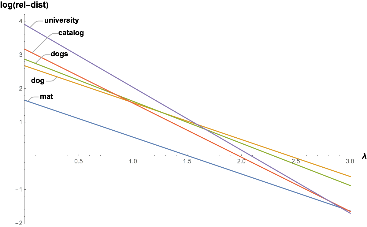
Figure 1 Relative distance (log scale) from “cat” versus λ for some sample words

We can extend these ideas to groups of words instead of just pairs.

Word Groups

Before looking at ways to compare different groups of words, we should explicitly state two underlying assumptions we will use:

  1. The greater the phonetic distance (as described above) between two words, the less likely they are to be confused
  2. The number of phonemes in a word is a reasonable measure of the ‘cost’ of using (saying) the word

The first is the basis of the work above. We have implicitly assumed that the more differences in consonant features, vowel metrics and duration between words, the less likely the words will be confused. We can partly confirm this by our own experiences and partly by common sense. In reality, it is likely the degree of confusion between words is more nuanced, and shrouded in how our brains process and recognise sounds. However, for our purposes, the approach taken will have to suffice.

The second assumption is more straightforward. Although there are differences in the duration of individual phonemes, these tend to average out within a words. Further the transition between each phoneme also affects the duration of pronouncing the word. So the number of phonemes in a word is a reasonable measure of the cost associated with its reproduction.

Armed with these two assumptions, we can perform a cost/benefit analysis on groups of words. The cost is associated with the phoneme counts of the words, while the benefit is the phonetic separation achieved between them.

As a concrete example, let’s return to the six words used to represent the hexadecimal characters (A-F) discussed earlier.

Hex Words

The two tables below show the raw distance, and relative distance (λ=2), in parentheses, for each hexadecimal word pairings for the ISA and USPA abbreviations respectively.

ISA alpha (4) bravo (5) charlie (5) delta (5) echo (3) foxtrot (8)
alpha (4) 0.0 (0.00) 31.4 (1.55) 27.9 (1.38) 11.8 (0.58) 20.1 (1.64) 47.3 (1.31)
bravo (5) 0.0 (0.00) 29.9 (1.20) 28.8 (1.15) 21.3 (1.33) 46.4 (1.10)
charlie (5) 0.0 (0.00) 28.3 (1.13) 33.4 (2.09) 43.7 (1.03)
delta (5) 0.0 (0.00) 21.9 (1.37) 46.0 (1.09)
echo (3) 0.0 (0.00) 47.8 (1.58)
foxtrot (8) 0.0 (0.00)

Table 13 Raw and relative distance (λ=2) of the ISA hex words

USPA able (4) baker (4) charlie (5) dog (3) easy (3) fox (4)
able (4) 0.0 (0.00) 18.2 (1.14) 34.0 (1.68) 24.0 (1.96) 18.4 (1.50) 29.4 (1.84)
baker (4) 0.0 (0.00) 34.0 (1.68) 22.0 (1.79) 22.0 (1.79) 23.1 (1.44)
charlie (5) 0.0 (0.00) 29.5 (1.85) 28.2 (1.76) 22.4 (1.11)
dog (3) 0.0 (0.00) 26.5 (2.95) 18.9 (1.54)
easy (3) 0.0 (0.00) 32.2 (2.63)
fox (4) 0.0 (0.00)

Table 14 Raw and relative distance (λ=2) of the USPA hex words

The question is how best to compare these two schemes and, indeed, schemes in general?

As suggested above, we want to maximise the benefit/cost ratio (or minimise the cost/benefit ratio) where benefit is some function of distance and cost some function of the number of phonemes. We also may want to consider the frequency or probability of words, that is, how often a word (or its associated letter) occurs. For hexadecimals, and many other real life scenarios (e.g call signs), this is expected to be approximately the same for each letter/word. But in some contexts, particular letter/words may be used more frequently than others.

Cost

Let’s start with the cost side of the equation. As we are assuming the cost is proportional to the number of phonemes in the word, the cost of saying the entire set of words is the sum of the probability (p) multiplied by the phoneme count (c) of each word.

cost = p1c1 + p2c2 + … + pncn = Σpici
where:
pi = probability of wordi (or its associated letter) occurring
ci = phoneme count for wordi
Note: p1 + p2 + … + pn = Σpi = 1

When the probability of each word is equally likely, as in the case of hexadecimal letters, pi = 1/n and the cost equation becomes a simple arithmetic mean:

cost = (1/n)c1 + (1/n)c2 + … + (1/n)cn = Σ(1/n)ci = Σci / n

This is a simple and effective cost measure. It would be possible to emphasis, and penalise, more costly (longer) words by using the generalised or power mean. It raises each value to some power before summing them. This inflates larger values and increases their relative contribution to the sum (assuming the exponent is greater than one). To normalise the result, the root is taken to the same power as shown below:

cost = (Σpiciτ)1/τ
or for pi = 1/n
cost = (Σ(1/n)ciτ)1/τ = (Σciτ/n)1/τ
where:
τ = constant
Note when τ=1, cost = Σci/n (as above)

However, for our purposes we will stick to the simple arithmetic mean of the phoneme counts.

Benefit

Now let’s consider the benefit side of the equation for a group of words.

If there are n words in the group, each word has n-1 neighbours and n-1 corresponding distances to them. So there is a total of n(n-1)/2 distances between the n words. To simplify matters, we will focus on the distance between a word and its nearest neighbour. This is the minimum distance associate with each word. It can be interpreted as a measure of the likelihood the word will be confused with another. It also means we only need to consider n distances for the benefit equation.

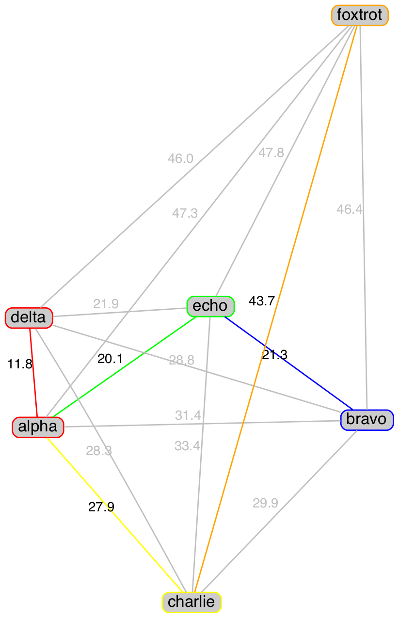
Figure 2 below shows graphs of the ISA and USPA words (nodes) with the links (edges) between them representing the raw distance from the table above. The minimum distance edges for each word are coloured along with their associated nodes (not to scale). It can be seen that the minimum minimum distance (red edge) is always shared between two nodes. While other nodes can either share or have their own minimum distance.

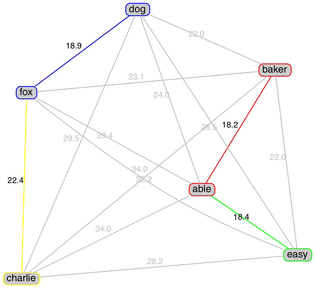
Figure 2 Minimum distance between ISA and USPA words

The result of this approach is that each letter/word is assigned a single distance value representing its worst case separation denoted d.

We can treat this minimum distance in a similar way to the cost phoneme count. Again the probability of the word being used can be similarly accommodated.

benefit = p1d1 + p2d2 + … + pndn = Σpidi
or for pi = 1/n
benefit = Σdi / n
where:
pi = probability of wordi (or its associated letter) occurring
di = distance between wordi and its nearest neighbour
Note: p1 + p2 + … + pn = Σpi = 1

Of course there a many other ways the cost and benefit equations could be formulated. There is no “correct” approach, but each should provide similar general results–reducing the cost for shorter words and increasing the benefit for greater separation–with only the quantum varying.

Quality Measure

The ratio of benefit to cost provides a quality measure for a set of words. The better the separation the greater the quality. The shorter the words (few phonemes) the greater the quality. The sensitivity to word length can be tuned with the λ parameters as follows:

qualλ = Σpidi / (Σpici)λ
or for pi = 1/n
qualλ = (Σdi/n) / (Σci/n)λ

To simplify matters we will consider three “special” cases of the quality measure assuming equal likelihood of letters/words:

qual0 = Σdi/n
qual1 = (Σdi/n) / (Σci/n)
qual2 = (Σdi/n) / (Σci/n)2

The first (qual0) is just the average minimum distance. It takes no account of the length of the words. Some constraint on the word length can be externally imposed by limiting the length of the candidate words available for selection.

The second (qual1) is the average minimum distance per phoneme. It takes basic account of the word length meaning longer words are not necessarily better than shorter ones but it places no particular penalty on longer words.

The last (qual2) places more emphasis on word length by penalising longer words. This is the most useful for our purposes as it represents the most economic measure.

We are now in a position to assess the two hexadecimal scheme above using these quality measures:

Scheme avg-phs qual0 qual1 qual2
ISA 5.00 22.76 4.55 0.91
USPA 3.83 19.18 5.00 1.31

Table 15 Hex word quality comparison

These results show that while the average minimum distance (qual0) for ISA are greater than USPA, USPA improves as λ increases because its average phoneme count is significantly smaller. These figures suggest that for hexadecimal words, at least, USPA is a significantly more economic scheme (by about 44%).

We will look at some alternative hexadecimal schemes later that have even better economy. Before we can create new schemes, however, we need a source of candidate words.

Candidate Words

For each letter of the alphabet we need a set of suitable words to represent it. The words must:

  1. Start with that letter (i.e. p for pot)
  2. Sound the letter as expected (i.e. p for pot but not p for physics nor e for europe)

To achieve the second condition, an acceptable first phoneme (or phonemes) is assigned for each letter. The following table show the proposed phoneme mapping.

Letter Phoneme(s)
a AE, EY
b B
c CH
d D
e EH, IY
f F
g G
h HH
i AY, IH
j JH
k K
l L
m M
 
Letter Phoneme(s)
n N
o AO, OW
p P
q K
r R
s S
t T
u AH, Y
v V
w W
x EH
y Y
z Z

Table 16 Initial word phoneme(s) for each letter

Note:

  1. There can be multiple phonemes to cover the case where a vowel, for example, sounds differently at the beginning of a word, for example, echo (EH) and easy (IY)
  2. The letter C uses the CH sound (as in check) instead of the K sound (as in cat) to distinguish it from the letter K which uses the K sound (as in kite)
  3. The letter X is a special case, as it invariably sounds like Z when used at the start of a word (e.g. xenon, xerox and xylophone). The one notable exception is x-ray which perforce will be used for the letter X.

Using the first letter and phonemes listed above we can assign words to letters. However, there are a few challenges in creating an suitable list of candidate words. Many of the words in the CMU are not suitable for various reasons and would make poor candidate words. For example, words that fall into any of the following categories may not be considered suitable:

  • Uncommon, obscure, archaic or foreign
  • Derogatory, racist, sexist, rude, indecent, swearwords, slang or intimate
  • Negative, depressing, anti-social
  • Technical or specialist in nature such as anatomical or botanical terms
  • Warning or emergency (e.g. fire, help, danger)
  • Numbers (e.g. one, two, …)
  • Place names such as countries, cities, rivers, etc.
  • Personal names (although these can be useful because they are often well known)
  • Company names, trademarks or product names (with possible legal implications)
  • Non root words (e.g plurals and other derivatives)
  • Religious, sacred or iconic
  • Abbreviations, acronyms or colloquial terms
  • Homonyms and homophones
  • Overly short or long words

This list is probably not exhaustive, in short, there are many and varied reasons to exclude words. Perhaps it is easier to define acceptable words as: common simple root words with a neutral or positive character that are unlikely to be offensive or symbolic to most people.

Consideration as to how the words will be used is also important. If they are for ad hoc use, in casual situations without a prior formal agreement, common and familiar words will be more effective. However, if the scheme is going to be used by a formal agreement between parties (e.g. ISA), it is more acceptable to use less common words as they will be familiar and expected by the parties involved. Indeed, somewhat obscure words may even be preferred as they are more readily recognisable as letter substitutes.

The CMU dictionary is full of words that would be caught in the unsuitable categories above. In particular, it has a large number of abbreviations, proper nouns and derivations. So as a more concise and manageable source of words we will use Google 10,000 most common English words as a base source. Of course the Google words also contain many words that fall into the undesirable categories above. As a result, a number of words have been excluded from the Google set to produce a subset for use in the examples below.

Alternative Hexadecimal Word Sets

Can we find alternative hexadecimal word sets to ISA and USPA that produce a higher quality result?

A simple approach would be to try every combination of the words representing the letters A-F and select the combination with the highest quality score. A little thought will reveal this has complexity scaling problems. If we assume about 10,000 / 26 (approx. 385) words per letter, there will be around 3856 or 3.25 x 10¹⁵ word combinations to analyse. Searching this entire solution space is problematic even with a fast computer and would be impossible with larger word groups like A-Z for the full alphabet.

Rather than looking for the optimal solution, we can find a sub-optimal, but hopefully still good solution, by reducing the size of the search. One simple approach is to:

  1. Select a word at random for each letter from the word candidates.
  2. Order the words from smallest to largest based on their minimum distance (i.e. distance to their nearest neighbour). When this is equal (which always occurs at least once) order by the number of candidate words available, least to most. So select the word with the closest neighbour and least number of alternative words first.
  3. For the selected word, try replacing it with each of the available alternative words from the candidate words. Calculate the resulting quality measure for the new word set and select the best alternative word based on this measure, or leave the current word if no improved word can be found.
  4. Repeat the above step for each word in turn.
  5. If there are no improvement found for any word finish, otherwise loop back to Step 2.

This is a simple form of gradient accent where each dimension (letter/word) is examined in turn for “higher ground”. Once no further improvement can be found we have reached a local maximum. By repeating the process for different random starting points we can search for better local maximums.

Some results from applying this approach to candidate words restricted to 3-5 phonemes using our three quality measures above (qual0, qual1 and qual2) are shown below in Tables 17, 18 and 19 respectively.

Local Maximum λ=0 (Hex35-λ0)

Hex35-λ0 april (5) balloon (5) charter (5) donate (5) energy (5) frank (5)
april (5) 0.0 (0.00) 31.8 (1.27) 34.4 (1.38) 34.1 (1.36) 33.9 (1.35) 32.3 (1.29)
balloon (5) 0.0 (0.00) 34.5 (1.38) 30.5 (1.22) 32.6 (1.30) 32.2 (1.29)
charter (5) 0.0 (0.00) 36.9 (1.47) 37.4 (1.50) 33.8 (1.35)
donate (5) 0.0 (0.00) 32.0 (1.28) 35.1 (1.40)
energy (5) 0.0 (0.00) 33.7 (1.35)
frank (5) 0.0 (0.00)

Table 17 Sample qual0 local maximum for hex words using 3-5 phonemes

Local Maximum λ=1 (Hex35-λ1)

Hex35-λ1 april (5) balloon (5) charter (5) donate (5) energy (5) frank (5)
april (5) 0.0 (0.00) 31.8 (1.27) 34.4 (1.38) 34.1 (1.36) 33.9 (1.35) 32.3 (1.29)
balloon (5) 0.0 (0.00) 34.5 (1.38) 30.5 (1.22) 32.6 (1.30) 32.2 (1.29)
charter (5) 0.0 (0.00) 36.9 (1.47) 37.4 (1.50) 33.8 (1.35)
donate (5) 0.0 (0.00) 32.0 (1.28) 35.1 (1.40)
energy (5) 0.0 (0.00) 33.7 (1.35)
frank (5) 0.0 (0.00)

Table 18 Sample qual1 local maximum for hex words using 3-5 phonemes

Local Maximum λ=2 (Hex35-λ2)

Hex35-λ2 april (5) balloon (5) charter (5) donate (5) energy (5) frank (5)
april (5) 0.0 (0.00) 31.8 (1.27) 34.4 (1.38) 34.1 (1.36) 33.9 (1.35) 32.3 (1.29)
balloon (5) 0.0 (0.00) 34.5 (1.38) 30.5 (1.22) 32.6 (1.30) 32.2 (1.29)
charter (5) 0.0 (0.00) 36.9 (1.47) 37.4 (1.50) 33.8 (1.35)
donate (5) 0.0 (0.00) 32.0 (1.28) 35.1 (1.40)
energy (5) 0.0 (0.00) 33.7 (1.35)
frank (5) 0.0 (0.00)

Table 19 Sample qual2 local maximum for hex words using 3-5 phonemes

The Hex35-λ0 solution optimises for qual0 where word length is ignored, so it only requires maximising the distance between words. Hence the result uses the longest words available – in this case five phonemes.

The Hex35-λ1 solution optimises for qual1, where the distance per phoneme is important, so the word length is essentially irrelevant. As a result we see a variety of word lengths.

Finally for the Hex35-λ2 solution which optimises for qual2, the word length penalises the result more and the solution favours words with the smallest phoneme count (while still trying to maximise separation distances).

Table 20 below compares these three local maximum solutions with the ISA and USPA schemes.

Scheme avg-phs qual0 qual1 qual2
ISA 5.00 22.76 4.55 0.91
USPA 3.83 19.18 5.00 1.31
Hex35-λ0 5.00 31.80 6.36 1.27
Hex35-λ1 4.17 29.15 7.00 1.68
Hex35-λ2 3.00 21.39 7.13 2.38

Table 20 Comparison of ISA, USPA and three local maximum word sets

We can see that the generated solutions deliver significantly better results in their quality category (highlighted cells) than either ISA or USPA. It also highlights that the solution produced using the local maximum procedure above is not necessarily the true maximum solution. The Hex35-λ2 word set is actually a better solution than the Hex35-λ1 word set for the qual1 measure. So Hex35-λ1 is clearly sub-optimal.

These generated word solutions are, of course, only one example of many possible word combinations that also score highly. Listed below is Hex35-λ2 and some other results with high qual2 scores in descending order:

  • act, bar, choice, duo, easy, fly (2.38)
  • arrow, bug, choice, duo, easy, fly (2.31)
  • arrow, booth, choice, dry, easy, far (2.30)
  • acre, beach, chuck, duo, end, fly (2.25)
  • amy, beach, choice, dry, echo, far (2.24)
  • ask, beach, choice, duo, era, fly (2.23)
  • annie, blue, choice, dock, east, fill (2.21)
  • arrow, bouquet, chase, door, easy, fly (2.15)
  • alloy, blue, chief, doll, end, folk (2.12)

Finally, as a baseline of sorts, let’s include a random sample of words with 3-5 phoneme counts. Table 21 below includes the average results (rand-35) of 1000 words sets drawn randomly from the same 3-5 phoneme word pool used by the local maximum solutions.

Scheme avg-phs qual0 qual1 qual2
ISA 5.00 22.76 4.55 0.91
USPA 3.83 19.18 5.00 1.31
Hex35-λ0 5.00 31.80 6.36 1.27
Hex35-λ1 4.17 29.15 7.00 1.68
Hex35-λ2 3.00 21.39 7.13 2.38
rand-35 4.04 18.86 4.67 1.16

Table 21 Includes average results from 1000 random samples taken from 3-5 phoneme words

It is interesting to note that for the six hexadecimal letters, ISA scores worse than a random sample on two of the three quality measures. USPA is marginally better on all three. All the constructed word sets score significantly better than the random samples for their optimised measure, and indeed better for the other measures as well.

Full English Alphabet

The methods used above can be extended to the entire 26 letters of the English alphabet. First lets compare the full ISA and USPA schemes with the average of 1000 random samples take from the 3-5 phoneme word pool in the same way we did for the hexadecimal case.

Scheme avg-phs qual0 qual1 qual2
ISA 4.96 20.07 4.05 0.82
USPA 3.81 14.82 3.89 1.02
rand-35 4.02 14.68 3.65 0.91

Table 22 Comparison of full ISA, USPA and average random sample from 3-5 phoneme words

The ISA scheme results are better here than the hexadecimal case for qual0 and qual1 against both USPA and the random samples. However for qual2 it falls below both. This reflects the significantly longer words used in ISA, averaging 4.96 phonemes compared with USPA’s 3.81 and 4.02 for the random samples.

Strangely, ISA has a number of words with the same ending sound. It has six words ending in AH, five in OW and three in ER and IY:

  • AH: alpha, delta, india, lima, papa, sierra
  • OW: bravo, echo, kilo, romeo, tango
  • ER: november, oscar, victor (noting ER is quite close to AH)
  • IY: charlie, whiskey, yankee

It is not clear whether this was by design or a coincidence, but it reduces its quality results as defined above. In comparison, USPA has five words ending in ER with all the remaining only one or two words:

  • ER: baker, peter, roger, sugar, victor

The full “histogram” of finals sounds (ordered high to low) for each is:

  • ISA: 6 5 3 3 2 2 1 1 1 1 1
  • USPA: 5 2 2 2 2 2 2 1 1 1 1 1 1 1 1 1

Constructed Alternatives

The same local maximum approach used for hexadecimal words above can be applied to the entire alphabet (A-Z). It produces a wider variety of possible solutions. Most have a mixture of “good” and “not-so-good” words based the categories above. One of the main issues is whether to include personal names (e.g. John, Kate, Howard, etc.). The upside is that names provide a richer set of phoneme combinations and increase the available word pool. The down side is that names are not standard english (i.e. not generally found in dictionaries) and some are more familiar than others to the general population. I’ve chosen to include them in this case.

Table 23 below shows two examples of local maximums for each of our three quality measures (labelled -a and -b). All words are again drawn from the 3-5 phoneme word pool.

Scheme avg-phs qual0 qual1 qual2 Words
ISA 4.96 20.07 4.05 0.82 alpha, bravo, charlie, delta, echo, foxtrot, golf, hotel, india, juliet, kilo, lima, mike, november, oscar, papa, quebec, romeo, sierra, tango, uniform, victor, whiskey, x-ray, yankee, zulu
USPA 3.81 14.82 3.89 1.02 able, baker, charlie, dog, easy, fox, george, how, item, jig, king, love, mike, nan, oboe, peter, queen, roger, sugar, tare, uncle, victor, william, x-ray, yoke, zebra
Full35-λ0-a 4.81 24.68 5.13 1.07 avenue, brother, charter, dial, ethics, future, ground, highway, input, joseph, kitchen, lottery, module, nylon, orange, piano, query, ratio, strong, tuesday, unique, value, willow, x-ray, young, zebra
Full35-λ0-b 4.81 24.38 5.07 1.05 alpine, blink, chester, direct, energy, future, grammar, hood, invoice, joel, kevin, locate, mature, nylon, orange, pottery, query, ratio, strong, teenage, uncle, venue, willow, x-ray, yard, zebra
Full35-λ1-a 4.23 22.72 5.37 1.27 address, book, choice, diana, eagle, flower, glory, heather, inch, july, katie, leo, marsh, nylon, ozone, pottery, queen, rainbow, spa, troops, unique, virtue, walter, x-ray, yoga, zebra
Full35-λ1-b 4.12 21.81 5.30 1.29 alpine, binary, choice, draw, eric, flyer, gourmet, hull, ink, johnny, kitchen, launch, marco, neon, over, poster, query, ratio, ski, tooth, unique, virtue, wage, x-ray, yellow, zebra
Full35-λ2-a 3.19 15.70 4.92 1.54 alloy, bull, chess, draw, easy, fog, garage, ham, ink, joke, keep, leo, more, nail, oboe, patch, quite, ridge, spa, town, under, view, wire, x-ray, young, zoom
Full35-λ2-b 3.27 15.88 4.86 1.49 alloy, beach, check, door, easy, file, grow, house, ink, join, kate, leo, myth, nest, old, poker, queen, roof, spa, top, under, view, wire, x-ray, young, zulu

Table 23 Comparison of full ISA, USPA and two local maximums optimised for λ=0, 1 and 2

Clearly it is possible to find word sets that achieve better results than both ISA and USPA using the distance measures defined in this blog. In fact, the problem is choosing between the large number of good solutions available.

Appendix D lists some high scoring word sets using different criteria for candidate word pools and quality measures. I’ll leave it to the reader to choose their favourite.

Conclusion

The idea of using a quantitative measure to evaluate, and generate, spelling alphabets seems like a relatively straightforward exercise. However, as this post demonstrates, there are a number of complexities that make it more challenging than expected. These include:

  • Mapping letters to words and their associated phonemes
  • Defining a distance (i.e. difference) measure between phonemes
  • Defining a distance measure between two words (i.e. two phoneme sequences)
  • Defining a distance and quality measure between two groups of words
  • Determining a pool of candidate words (for generation)
  • Selecting words from the candidate pool to maximise a quality measure

An attempt to systematically address each of these is included in this blog.

Perhaps the most innovative element is the use of discrete convolution to measure the phonetic distance between two words. This allows different phoneme durations to be accommodated in a natural way. How well the word differences, determined by this convolution, compare with actual human perception is an open question. However it does provide a robust quantitative comparison method.

The analysis does suggest that ISA is far from optimal based on the presented measures. Even without this analysis its strange preference for words ending with AH (6 instances) and OW (5 instances) phonemes is a sign that improvement is possible. Of course its near universal adoption makes any change all but impossible. However for informal use, readers could select any of the options in Appendix D and be confident that there is at least some science behind their choice.


APPENDICES


Appendix A

Distance Normalisation and Scaling

Given a set of m points P ⊂ ℝn and a set of weights {w1, w2, …, wn} that scale each of the n dimensions, the Euclidean distance function for any two points x, y ∈ P is:

d(x,y) = √([w1(x1-y1)]2 + [w2(x2-y2)]2 + … + [wn(xn-yn)]2)

The requirement is to adjust the weights (wi > 0) so that in general terms:

  1. The contribution of each dimension is about equal that is:
    • inflate dimensions that are numerically small compared with others
    • deflate dimensions that are numerically large compared with others
    • don’t just make a wi very small and convert the problem from ℝn to ℝn-1
  2. The maximum distance between any two points is 1.0
  3. The average (mean) distance between points is 0.5

More formally:

1. Σx,y∈P w1|x1-y1| ≈ Σx,y∈P w1|x2-y2| ≈ … ≈ Σx,y∈P wn|xn-yn|
2. maxx,y∈P d(x,y) = 1.0
3. Σx,y∈P d(x,y) / m2 = 0.5

Firstly note that the entire space can be scaled by a single factor, k, to expand or contract it. This factor can thus be used to achieve either condition 2, by scaling the maximum distance to 1.0, or, condition 3, by scaling the average to be 0.5, but not both. To achieve both we need to apply a non-linear monotonic function to the weights. Here we choose to raise them to a power r.

The first condition gives the following equation for the weights:

Σx,y∈P w1|x1-y1| = Σx,y∈P w2|x2-y2| = … = Σx,y∈P wn|xn-yn| = 1 (say)
w1 Σx,y∈P|x1-y1| = w2 Σx,y∈P|x2-y2| = … = wn Σx,y∈P|xn-yn| = 1
wi = 1 / Σx,y∈P|xi-yi|
Apply a non-linear scaling power r we get:
wi = (1/Σx,y∈P|xi-yi|)r
Apply a uniform scaling factor k gives:
wi = k(1/Σx,y∈P|xi-yi|)r
or
wi = k(1/Δi)r = k/Δir
where:
Δi = Σx,y∈P |xi-yi|

Substituting this back into the original distance equation gives:

d(x,y) = √([k(x1-y1)/Δ1r]2 + … + [k(xn-yn)/Δnr]2)
or
d(x,y) = k√([(x1-y1)/Δ1r]2 + … + [(xn-yn)/Δnr]2)

Now for any given power r (eg. r = 1.0) it is easy (with a computer :) to determine k so that the average distance is 0.5 using:

avg = Σx,y∈P d(x,y) / m2 = 0.5
Σx,y∈P k√([(x1-y1)/Δ1r]2 + … + [(xn-yn)/Δnr]2) / m2 = 0.5
x,y∈P √([(x1-y1)/Δ1r]2 + … + [(xn-yn)/Δnr]2) = 0.5m2
k = 0.5m2 / Σx,y∈P √([(x1-y1)/Δ1r]2 + … + [(xn-yn)/Δnr]2)

Now, by inspection of the maximum distance, r can be adjusted to move it towards its target value of 1.0. Repeated iterations using a binary search (chop) approach allows r to be determined to any appropriate level of accuracy. Once r is determined, k is known and the final weights can be calculated.

This approach may not be the most efficient but as it only needs to be carried out once it is not that critical.

Appendix B

Mean Distance between a Point and a Line Segment

The distance between a point and a line segment can be calculated numerically or analytically. Numeric approach provides an approximation by dividing the line segments into a number of equally spaced points and taking the average of the distances from the point to the line segment sub-points. Increasing the number of sub-points improves the accuracy of the result.

The analytical solution proves to be a bit trickier than one might expect. One approach is given below although alternative solutions that are more straightforward may be possible.

Consider four points P, Q, R and S in ℝn and their corresponding vectors p, q, r and s. R and S are the start and end of a line segment. Q is a point on the line segment and P is the reference point. The Euclidean distance between P and Q, or the magnitude of pq (written pq) is d as shown in the diagram below.

We want the mean (average) distance between P and the line segment RS.

Using the parametric definition of Q we have q = r + x(sr) so that as x ranges from 0 to 1, q ranges from r to s.

Define the distance function, d(x), to be the magnitude of PQ (pq) for a given x, then the mean distance is the integral of d(x) between 0 and 1. Below we use standard vector dot product algebra to expand d(x) in terms of r, s and p, and then group them in powers of x to form a quadratic equation.

Let q = r + x(sr)
d(x) = pq = √(pq).(pq)
  = √(p – (r+x(sr))).(p – (r+x(sr)))
  = √((pr) – x(sr)).((pr) – x(sr))
  = √(sr).(sr)x2 – 2(sr).(pr)x + (pr).(pr)
  = √(ax2 + bx + c)
where:
a = (sr).(sr)
b = -2(sr).(pr)
c = (pr).(pr)
So we have:
avg-dist = ∫01 d(x) dx = ∫01 √(ax2 + bx + c) dx

The integral above is a bit messy but available from various mathematical applications or sites. The following is courtesy of WolframAlpha:

∫√(ax2 + bx + c) dx =
[(4ac-b2)log(2√(a)√(ax2+bx+c) + 2ax + b) + 2(2ax+b)√(a)√(ax2+bx+c)] / 8a3/2

The mean distance can thus be calculate by plugging in the values of a, b and c and subtracting the integral’s value at x=0 from its value at x=1.

After coding up both approaches, there was good agreement (better than 10-4) between them using 1000 sub-points for the numeric approximation.

Mean Distance between Two Line Segments

The approach taken above can be readily applied to the case of the mean distance between two line segments. Consider the following diagram.

Line segments TU and RS have parametric points P and Q on them respectively. Their corresponding parametric vectors (p and q) move from T to U and R to S as x varies from 0 to 1. As above, we define the distance d between P and Q in terms of x and integrate over the range 0 to 1 to get the average distance.

More formally:

Let p = t + x(ut), q = r + x(sr), giving
pq = (t + x(ut)) – (r + x(sr))
  = x((ut)-(sr)) + (tr)
d(x) = pq = √(pq).(pq)
  = √[((ut)-(sr)).((ut)-(sr))x2 + 2x((ut)-(sr)).(tr) + (tr).(tr)]
  = √(ax2 + bx + c)
where:
a = ((ut)-(sr)).((ut)-(sr))
b = 2((ut)-(sr)).(tr)
c = (tr).(tr)

We can plug these values into the integral above to calculate the result.

Appendix C

Coding Discrete Convolution

Coding the convolution of two strings (or any two sequences of discrete values) can appear a bit daunting. However it is actual straightforward if you:

  • reverse the second string
  • lay them out in a grid, with the first string at the top and the reversed second string on the left
  • calculate the value of each cell using the corresponding horizontal and vertical character (or sequence value)
  • sum each of the grid diagonals to get the final convolution value

It is even easier to program if you note that the diagonal cells all have the same index sum value (i.e. the sum of the two corresponding sequence indices). This index value can be used to group the cell results into diagonals for summing.

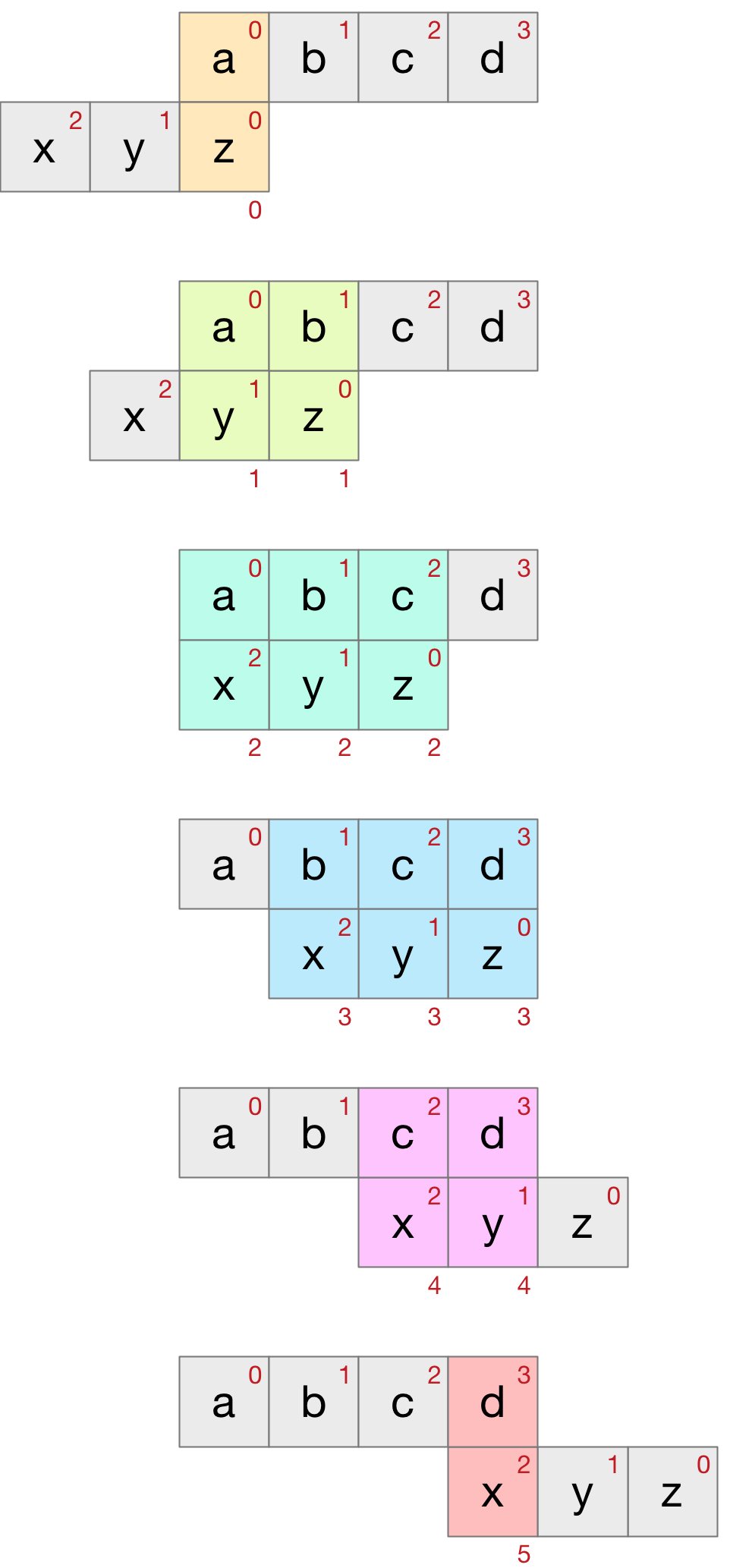
An example will make it clear. Consider the convolution of the two strings abcd and xyz. Using the above procedure we obtain a grid as follows:

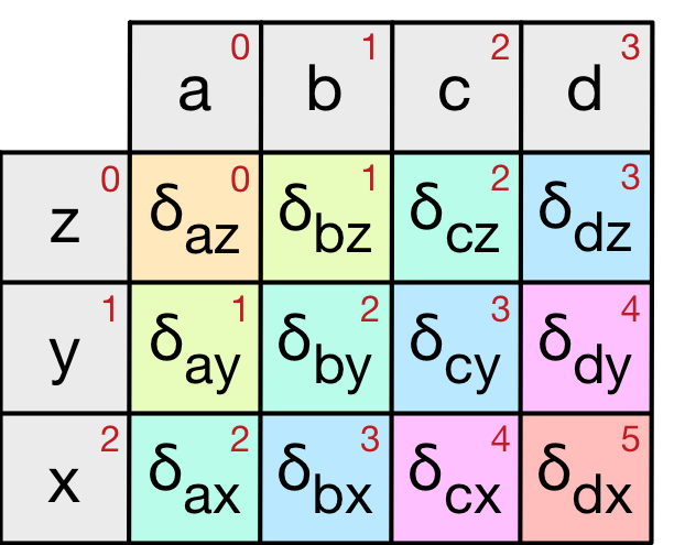
The xyz string is reversed to zyx and the δij value in the cells represent the distance between the i and j character (phoneme in our case). The small red numbers in the top right corner of the strings represents the index value of the phoneme in the string. The same numbers in the cells represent the sum of the indices of the two corresponding string phonemes. This sum can be used to programatically identify the diagonal associated with each cell. The diagonals have also been coloured for clarity. The convolution values are just the sum of the diagonals:

  • convolution0 = δaz
  • convolution1 = δay + δbz
  • convolution2 = δax + δby + δcz
  • convolution3 = δbx + δcy + δdz
  • convolution4 = δcx + δdy
  • convolution5 = δdx

These correspond to the string positions shown below as the two string pass each other.

Example Clojure code might look like:

(defn convolution
  "Convolution of two sequences applying the function 'conv-fn'
  to adjacent values and summing the results."
  [seq1 seq2 conv-fn]
  (let [vec1 (vec seq1)
        vec2 (vec (reverse seq2))
        res (reduce
              (fn [acc [i1 i2]]
                (let [cell (conv-fn (vec1 i1) (vec2 i2))]
                  (update acc (+ i1 i2) (fnil + 0) cell)))
              {}
              (for [i1 (range (count vec1))
                    i2 (range (count vec2))]
                [i1 i2]))]
    (vals (sort res))))

Appendix D

Generated Example Word Sets

The following are some generated word sets using different criteria for the length of the candidate words (phoneme count) and the quality setting (λ value).

Sample 4-phoneme word sets maximising qual0 (λ=0)

The following local maximum word sets use words with exactly four phonemes. Their raw distance (qual0) is shown in brackets.

  • alpha, boost, charm, diary, eric, flower, graph, hockey, icon, july, kilo, lounge, maria, neon, ozone, paper, queen, royal, score, today, under, virtue, wax, yoga, zinc (20.18)
  • aqua, black, charge, diary, epic, flour, growth, hockey, image, july, kind, lewis, maria, neon, ozone, paper, queen, royal, spray, trio, under, virtue, willow, yoga, zinc (20.15)
  • aqua, below, chance, diary, epic, flower, graph, hockey, image, joel, karl, launch, maria, neon, ozone, paper, queen, relay, scoop, trio, under, virtue, wealth, yoga, zinc (20.03)
  • asset, broad, change, diary, eagle, flour, golf, hockey, image, july, kerry, lewis, maria, neon, ozone, paper, queen, royal, spice, trio, under, virtue, willow, yoga, zinc (19.88)
  • aqua, bound, charge, deny, epic, flower, gamma, hobby, ivory, joel, kilo, lucy, mother, neon, ozone, paper, queen, relay, score, track, under, virtue, wealth, yoga, zinc (19.81)
  • aqua, bother, chart, deny, eagle, flour, group, health, ivory, joel, kerry, launch, movie, neon, office, parade, queen, relay, score, trio, under, virtue, willow, yoga, zinc (19.80)
  • aqua, breach, child, data, eric, flower, growth, howard, ivory, joel, kilo, launch, movie, neon, office, poker, quiz, rally, snap, today, under, virtue, wolf, yarn, zinc (19.73)
  • alpha, bloom, change, depot, every, father, guru, hollow, icon, july, kerry, louise, march, neon, ozone, price, quit, royal, score, trio, under, virtue, wax, yoga, zinc (19.69)
  • aqua, broad, change, diary, epic, flower, guru, hockey, image, joel, kept, luther, march, neon, ocean, paper, queen, relay, spice, trio, under, virtue, wolf, yellow, zinc (19.63)
  • alpha, below, charge, drag, eric, flower, guru, highway, icon, july, kept, louise, money, nature, ozone, poem, quiz, round, spray, trio, under, visa, wales, yoga, zinc (19.58)
  • alice, baker, change, dial, even, form, glad, health, ivory, july, kilo, louise, mother, neon, ozone, prior, quick, robbie, spouse, truth, under, virtue, wax, yoga, zinc (19.51)
  • asset, baker, change, drag, every, flower, ghost, health, image, july, kilo, laura, maria, neon, ozone, papa, quiz, royal, speech, today, under, virtue, worthy, yarn, zinc (19.50)
  • aqua, bloom, change, duty, eric, flower, graph, highway, image, july, kilo, louise, marsh, neon, often, poet, quiz, river, spray, trio, under, virtue, worthy, yoga, zinc (19.47)
  • aqua, block, change, depot, eagle, flower, guru, health, ivory, july, karl, louise, mother, navy, office, past, quit, ryan, spray, truth, under, virtue, willow, yoga, zinc (19.39)
  • asset, breath, change, diane, every, flower, guard, health, image, jewel, kilo, laura, movie, neighbour, ocean, poker, quote, rally, speech, today, under, virtue, wax, yeast, zinc (19.32)
  • aqua, boost, charge, diary, epic, flag, guru, hello, image, july, kind, laura, marine, never, ocean, paper, quote, royal, spray, trio, under, virtue, worthy, yield, zinc (19.13)

Sample 3-phoneme word sets maximising qual0 (λ=0)

The following local maximum word sets use words with exactly three phonemes. Their raw distance (qual0) is shown in brackets.

  • alloy, batch, cheap, door, easy, free, grow, height, ink, joke, ken, leo, myth, noise, oboe, pale, ross, spa, tower, view, wool, young, zoom (14.90)
  • alloy, batch, choice, draw, easy, file, gate, hear, ink, judge, kim, leo, more, neck, oboe, play, ross, spa, tower, view, wool, yoke, zoom (14.74)
  • alloy, batch, choice, duo, easy, fish, grey, hub, ink, jeep, ken, leo, mouth, nail, over, power, ross, spa, tall, view, wool, yoke, zoom (14.68)
  • alloy, bang, cheap, door, east, full, gauge, house, ion, joke, king, leo, mug, noise, oboe, power, ruth, spa, tree, view, watch, year, zen (14.65)
  • amy, batch, check, dog, era, free, grow, heath, ink, juice, keen, leo, mime, noise, oboe, power, ross, spa, tour, view, whale, young, zip (14.59)
  • alloy, beach, choice, duo, easy, file, grey, hair, ion, jam, kate, leo, merge, nut, over, power, rock, spa, tall, view, wing, yoke, zoom (14.58)
  • amy, beach, choice, draw, era, file, give, hall, ink, jar, kirk, leo, mouth, nan, oboe, play, race, spa, tower, view, watch, young, zoom (14.49)
  • amy, blue, chief, dry, era, full, gauge, heel, ink, joan, kirk, leo, mouth, nan, oboe, power, rod, ski, touch, voice, walk, youth, zip (14.49)
  • alloy, beach, choice, duo, easy, fame, grey, hood, ink, judge, kirk, long, mouth, near, oboe, poll, ruth, spa, tower, view, wife, yacht, zen (14.45)
  • alloy, bush, chat, draw, east, free, gauge, hull, issue, joke, kick, leo, mayor, neil, over, paul, rock, sky, touch, voice, worth, year, zen (14.43)
  • amy, bar, chief, dog, era, foam, grow, height, ink, jam, kirk, leo, match, noise, oboe, pale, rule, sky, tree, view, wire, young, zip (14.41)
  • arrow, beach, chat, down, easy, few, game, hood, ink, june, kiss, leo, merge, near, over, play, rock, spa, tall, voice, wire, yoke, zen (14.38)
  • alloy, batch, chase, dare, easy, firm, grey, hawk, ink, judge, keen, leo, moon, noise, oboe, power, ripe, spa, toll, view, whale, yacht, zip (14.35)
  • amy, ball, choice, debt, era, flow, give, hire, ink, jar, kirk, leo, mouth, neil, oboe, page, rope, spa, tree, view, watch, young, zoom (14.30)
  • alloy, bull, chase, deal, east, fare, grow, house, issue, joan, kirk, log, mayor, none, over, power, ram, spa, tree, void, watch, youth, zip (14.29)
  • annie, beth, chase, duo, echo, few, goal, hood, ink, jar, keen, layer, mouth, night, over, patch, run, spa, tree, voice, walk, year, zoom (14.26)
  • alloy, blue, cheap, dry, east, fog, guide, hull, ion, joke, king, leo, mouth, net, oboe, power, rush, ski, tall, voice, wage, year, zoom (14.13)
  • alloy, batch, chase, dose, east, fare, grow, hire, issue, judge, keen, leo, mouth, nerve, owen, push, ross, spa, tree, void, walk, youth, zip (14.12)
  • alloy, bush, chess, draw, east, few, gauge, hair, ion, june, kirk, lower, mouth, neil, oboe, play, ram, spa, tall, voice, watch, young, zip (14.10)
  • alloy, blue, cheese, down, east, fell, goal, hawk, iron, jar, king, leo, mayor, none, oboe, patch, ride, spa, tree, voice, wake, youth, zip (14.08)

Sample 3-4 phoneme word sets maximising qual2 (λ=2)

The following local maximum word sets use words with three or four phonemes. Their qual2 (λ=2) is shown in brackets.

  • alloy, beth, chip, draw, easy, free, girl, hire, ink, join, keen, leo, mouth, near, oboe, page, quote, run, sky, talk, under, view, wood, yacht, zoom (1.56)
  • alloy, bell, choice, draw, easy, few, goal, hawk, ink, jack, kind, leo, mouth, neighbor, oboe, play, queen, rich, spa, teeth, under, virtue, wire, yacht, zoom (1.56)
  • alloy, beth, chase, draw, easy, file, goal, hawk, ink, job, keep, leo, match, noise, oboe, play, quote, rear, spa, tower, under, view, wood, young, zoom (1.56)
  • alloy, beef, chain, draw, easy, free, good, hire, ink, joke, kept, leo, mouth, nature, oboe, paul, quote, rock, sky, touch, under, view, worm, year, zoom (1.56)
  • alloy, batch, choice, doug, easy, fall, grow, height, ink, jeep, kim, leo, mail, never, oboe, play, queen, ross, spa, town, under, view, wool, yoke, zoom (1.56)
  • alloy, bench, cheat, draw, easy, feature, girl, house, ink, join, kilo, leo, myth, north, oboe, play, quick, rock, spa, tower, under, view, wage, young, zoom (1.55)
  • alloy, blue, chair, doug, easy, feature, grey, hall, ion, joke, kim, leo, merge, nail, oboe, power, queen, rack, spa, tooth, under, voice, wood, yacht, zinc (1.55)
  • amy, beth, choice, depot, era, full, grey, home, ink, july, keen, leo, more, none, oboe, power, quote, rack, spa, tooth, under, view, wage, yacht, zip (1.55)
  • alloy, bath, choice, down, east, free, goal, hawk, icon, jake, keen, leo, moon, nature, oboe, push, quote, ross, spa, today, under, view, wire, young, zip (1.55)
  • alloy, bull, choice, dog, easy, fiber, grow, hire, ink, jack, karl, leo, myth, noon, oboe, play, queen, rope, spa, town, under, view, wage, young, zen (1.54)
  • alloy, beth, chat, draw, easy, free, gauge, hall, ink, joke, kerry, leo, mayor, near, oboe, peak, quiz, rock, sky, touch, under, voice, wine, yard, zoom (1.53)
  • alloy, box, cheap, dash, east, file, grey, home, issue, jar, ken, leo, myth, nature, old, power, quote, roof, spa, tour, under, voice, wall, young, zinc (1.53)
  • alloy, bull, chase, draw, easy, feature, grey, hawk, ink, job, keen, leo, match, noise, oboe, pair, quick, roof, spa, tower, under, view, won, yard, zip (1.52)
  • alloy, ball, cheap, draw, east, few, gary, hood, iron, june, kind, leo, major, none, oboe, pitch, quick, rock, ski, tower, under, voice, worth, yoke, zinc (1.52)
  • apt, book, chief, draw, easy, fall, guru, house, ivory, jack, ken, leo, mail, noise, old, play, queen, ridge, spa, touch, under, view, wire, yacht, zinc (1.52)
  • alloy, bull, choose, dome, east, feature, grow, hear, issue, jake, kerry, leo, more, noise, oboe, play, queen, rug, spa, tower, under, van, watch, youth, zip (1.52)
  • alloy, bull, choice, duo, east, free, gale, hawk, issue, jack, ken, logo, merge, north, owen, power, quote, ross, spa, teach, under, visa, wife, young, zip (1.51)
  • alloy, bull, choose, duo, east, fairy, guard, hat, icon, join, keep, log, mouth, nature, oboe, poker, quote, rich, spa, tray, under, view, wire, young, zinc (1.50)
  • amy, blue, chain, dock, east, fall, grey, hub, isaac, july, kick, leo, memo, neil, old, patch, quote, rare, spa, tiger, under, voice, wire, youth, zinc (1.50)
  • act, bull, chat, door, emma, foam, grow, house, issue, judge, ken, leo, meat, noise, owen, play, quick, rock, spa, taylor, under, vary, wire, youth, zinc (1.49)

Sample 4-5 phoneme word sets maximising qual1.5 (λ=1.5)

The following local maximum word sets use words with four or five phonemes. Their qual1.5 (λ=1.5) is shown in brackets.

  • alpha, bloom, child, dark, every, flour, graph, hockey, icon, july, kevin, launch, mother, neon, oscar, paper, quit, royal, score, trio, unique, virtue, willow, x-ray, yoga, zinc (2.50)
  • amber, block, child, dual, eden, fridge, growth, holly, indoor, july, kilo, launch, marco, nylon, ozone, piano, query, ratio, spouse, taxi, unique, virtue, weather, x-ray, yoga, zinc (2.48)
  • alex, bound, charge, diary, enter, flower, glass, hockey, image, july, kilo, leon, maria, nursery, ozone, prove, quiz, radar, score, tango, unique, virtue, wealth, x-ray, yoga, zinc (2.48)
  • anchor, bother, cherry, diary, ethics, flower, gourmet, horse, image, july, karma, lounge, marine, nylon, ozone, poem, quit, ratio, school, track, unique, virtue, willow, x-ray, yoga, zebra (2.46)
  • aqua, below, change, dairy, every, flower, grill, host, image, july, kitchen, louise, mother, neon, office, proper, quote, royal, speech, tank, under, virtue, width, x-ray, yarn, zebra (2.46)
  • alpha, baby, change, dial, eric, flour, group, hammer, icon, july, kilo, louise, maria, north, ozone, poster, quiz, research, stock, tango, unique, virtue, want, x-ray, yoga, zinc (2.45)
  • alpha, birthday, change, derek, emily, flower, ghost, highway, image, july, kilo, large, marine, nylon, ozone, patio, quiz, royal, spot, truth, unique, virtue, water, x-ray, yield, zinc (2.45)
  • amateur, block, change, dual, epic, fully, growth, howard, ivory, jackie, kitchen, lucia, morris, neon, ozone, post, queen, recall, spice, trio, under, virtue, willow, x-ray, yard, zinc (2.45)
  • alex, bother, chapter, daisy, every, flag, growth, heater, invoice, july, karma, louise, most, neon, often, powder, quit, royal, score, trio, unique, virtue, wild, x-ray, yellow, zinc (2.45)
  • alex, beneath, charlie, decade, every, flower, greg, hockey, icon, july, kind, louise, major, neon, ozone, proper, query, royal, scoop, trio, under, virtue, warm, x-ray, yellow, zinc (2.44)
  • alex, bound, charge, daily, eagle, father, group, hockey, ivory, july, kitchen, logo, matthew, neon, office, pressure, quiz, royal, stock, trio, under, viking, warm, x-ray, yellow, zinc (2.44)
  • alpine, blake, charter, dual, every, forge, growth, howard, india, july, kitchen, lobby, month, nylon, office, prior, query, railway, scott, tank, uncle, virtue, willow, x-ray, yoga, zebra (2.43)
  • aqua, brush, change, donor, eric, flyer, ground, howard, ivory, joel, kitchen, louise, manage, north, oscar, papa, query, ratio, spoke, today, unique, virtue, willow, x-ray, yeast, zinc (2.41)
  • alice, bunch, chart, dating, emily, flower, growth, hockey, input, july, kilo, lewis, module, neon, order, parade, queen, rank, score, trio, unique, value, weather, x-ray, yoga, zebra (2.41)
  • aqua, block, chance, daughter, enzyme, flyer, growth, howard, image, jewel, karl, larry, marine, nylon, oscar, piano, quit, railway, spouse, trio, unique, virtue, willow, x-ray, yeast, zinc (2.41)
  • april, brad, change, daily, every, flower, gather, hockey, item, july, karl, laura, mold, neon, ozone, pillow, quote, royal, speech, tango, under, virtue, wealth, x-ray, yeast, zinc (2.41)
  • andy, box, channel, dual, even, flyer, graph, horn, icon, july, kilo, lounge, major, notice, oscar, parade, quick, rubber, speech, tango, unique, virtue, worthy, x-ray, yield, zinc (2.41)
  • alpha, body, charge, dual, emily, folder, guitar, highway, image, joint, kilo, luther, maria, nursery, ozone, piano, quiz, ratio, speech, trout, unique, virtue, warm, x-ray, yeast, zinc (2.41)
  • alex, block, change, decor, enzyme, flyer, grill, hobby, image, jewel, karma, leon, module, nursery, oscar, parade, quote, rover, speech, tango, unique, viking, width, x-ray, yellow, zebra (2.40)
  • after, broad, charge, delay, eric, future, gather, hockey, icon, jamie, kitchen, louise, month, neon, oval, parade, quiz, rainbow, solo, trio, unique, virtue, wolf, x-ray, yeast, zinc (2.38)

Alternative Star Trek Warp Speed Scale and Related Equations

Alternative Warp Speed Scale

At the risk–hopefully not too great–of offending Star Trek enthusiasts and traditionalists, it seems that a simple update to the Warp speed definitions would allow for more realistic exploration of space without departing unduly from the original concept.

The update would use a simple base-10 log scale. Log scales are often used in science and technology with Decibel and Richter scales being common examples.

Under this revision, a Starship’s speed or velocity (v) would be defined as:

v = 10w-1c …(1)
where:
v = velocity (speed)
w = Warp speed
c = speed of light

Equation 1 above uses w-1 (rather than just w) as the exponent to preserve Warp 1 as the speed of light (c), since 100 = 1, which is in keeping with existing scales and the general understanding of Warp speeds. Warp 2 becomes 10 times the speed of light, Warp 3 is 100 times, etc.

Table 1 is a comparison with existing Warp speed factors (multiples of the speed of light):

Warp TOS (w3) TNG/DS9/VOY Proposed (10w-1)
1 1 1 1
2 8 10 10
3 27 39 100
4 64 102 1000
5 125 214 10,000
6 216 392 100,000
7 343 656 1M
8 512 1024 10M
9 729 1516 100M
9.9 3053 794M
9.99 7912 977M
10 Not possible Not possible 1000M (see below)

Table 1 Comparison of Traditional and Proposed Warp Speed Factors

Series abbreviations:

  • TOS = The Original Series
  • TNG = The Next Generation
  • DS9 = Deep Space Nine
  • VOY = Voyager

The main advantages of the proposed approach are that it:

  • aligns reasonably well, and in some cases better, with time/distance in the TV/film series
  • makes the galaxy more navigable in human time frames
  • makes intergalactic travel plausible
  • would relax the somewhat artificial and tortured Warp 10 limit, however, this can be restored in a more mathematically rigorous way (see below)

While the proposed speeds are significantly greater than the standard scales, at least for higher Warp values, they fit more comfortably with the vast distances found in our Universe. For example, using the old scale (TNG say), to travel from Earth to the centre of our galaxy, about 25,000 light years, it would take over 16 years at Warp 9 and over 3 years at Warp 9.99.

Going to another (close) galaxy is simply implausible, taking 300 or more years at Warp 9.99. Given there are hundreds of billions of galaxies out there, it seems a bit limiting to restrict exploration to such a tiny fraction of the known universe.

By contrast, Table 2 below shows a distance and travel time chart for the proposed new scale.

Warp Local Planets Nearby stars Visible stars Federation Centre of galaxy Cross galaxy Nearby galaxies
(0.0005 ly) (50 ly) (500 ly) (5,000 ly) (25,000 ly) (100,000 ly) (5 Million ly)
1 4.4 hr 50.0 yr 500 yr 5,000 yr 25,000 yr 100,000 yr 5,000,000 yr
2 26.3 min 5.0 yr 50.0 yr 500 yr 2,500 yr 10,000 yr 500,000 yr
3 2.6 min 6.0 mth 5.0 yr 50.0 yr 250 yr 1,000 yr 50,000 yr
4 15.8 sec 2.6 wk 6.0 mth 5.0 yr 25.0 yr 100 yr 5,000 yr
5 1.6 sec 1.8 day 2.6 wk 6.0 mth 2.5 yr 10.0 yr 500 yr
6 0.16 sec 4.4 hr 1.8 day 2.6 wk 3.0 mth 1.0 yr 50.0 yr
7 16 msec 26.3 min 4.4 hr 1.8 day 1.3 wk 1.2 mth 5.0 yr
8 1.6 msec 2.6 min 26.3 min 4.4 hr 21.9 hr 3.6 day 6.0 mth
9 0.16 msec 15.8 sec 2.6 min 26.3 min 2.2 hr 8.8 hr 2.6 wk
10 0.016 msec 1.6 sec 15.8 sec 2.6 min 13.1 min 52.6 min 1.8 day

Table 2 Distance and Travel Times for the Proposed New Warp Speeds

Remembering that a scale is just that, a scale. It doesn’t mean that starships can reach these speeds or sustain them for extended periods. Indeed, standard cruising speed may be significantly less than full speed because of engine stress and energy efficiency.

The next section builds on these ideas by placing limits on Warp speed based on various criteria.

Warp Speed Constraints

To provide limits on the speed of Warp capable ships, and to stay faithful to the idea of a universal maximum Warp speed, for example Warp 10, we can introduce some constraints. One approach is a blend of relativistic and newtonian mechanics.

First, let’s assume that:

  1. The force required to move a ship though the Warp field is proportional to the square of its Warp speed, and,
  2. There is an universal maximum Warp speed (μ) similar to the speed of light in standard physics

Based on these two assumptions, the force (F) required to “push” through the Warp field can be written mathematically as:

F = aw2 / √(μ2-w2) …(2)
where:
F = force
a = constant
w = warp speed
μ = universal maximum warp speed

The numerator is the Warp squared factor from the first assumption above. The denominator is analogous to the Lorentz factor of special relativity which is usually written 1/√(c2-v2). It means the required force increases as the speed approaches the universal maximum Warp speed and becoming infinite at that maximum Warp speed. This meets the second assumption above and provides a robust mathematical underpinning of the limit.

Using the force definition from Equation 2 and the velocity from Equation 1, we can calculate the Power (P) required by a Warp engine to maintain a constant velocity using the standard relation:

  • Power (P) = Force (F) by velocity (v)

This gives:

P = Fv = acw210w-1 / √(μ2-w2) …(3)
where:
P = power
F = force
v = velocity (speed)
a = constant
c = speed of light
w = warp speed
μ = universal maximum warp speed

From Equation 3 the energy needed to travel a particular distance can be derived using the standard definitions:

  • distance (d) = velocity (v) by time (t)
  • Energy (E) = Power (P) by time (t)

This leads to the following energy equation:

d = vt
E = Pt = (Fv)t = F(vt) = Fd = adw2 / √(μ2-w2) …(4)
where:
E = energy
P = power
F = force
v = velocity (speed)
t = time
d = distance
a = constant
w = warp speed
μ = universal maximum warp speed

In addition to power and energy calculations, we can derive an equation for efficient defined as the distance travelled per unit of energy consumed (similar to fuel efficiency for motor vehicles). The efficiency (eff) equation follows directly from Equation 4:

eff = d/E = √(μ2-w2) / aw2 …(5)

Setting a Universal Maximum Warp (μ)

We can choose any Warp speed as the universal maximum, but let’s stay with convention and make μ=10.

The constant a in the above equations depends on the “units” we use to measure the various quantities. For simplicity, let’s make P=1 when w=1. We can put these values into the Power equation (3) above and solve for a as follows:

1 = ac12101-1 / √(102-12)
1 = ac / √(102-12)
ac = √(102-12) = √99
a = √99 / c

Then substituting a back into Equations 3 gives:

Pμ=10 = √99w210w-1 / √(100-w2) …(6)

Using the same approach for the Energy and Efficiency equations, namely:

  • Energy = 1 per unit distance (say 1 lightyear) when w = 1
  • Efficiency = 1 (100%) when w = 1

We get:

Eμ=10 = √99w2 / √(100-w2) per unit distance …(7)
effμ=10 = √(100-w2) / √99w2 …(8)

Table 3 below shows comparative results for Power, Energy and Efficiency for various Warp speeds based on Equations 6, 7 and 8. It also includes the time it would take to travel one light year at the given Warp speed as a reference.

Warp Power Energy per ly Efficiency (%) Time to travel 1 ly
1 1 1.0 100.00 1.0 yr
2 41 4.1 24.62 1.2 mth
3 939 9.4 10.65 3.6 day
4 17,370 17.4 5.76 8.8 hr
5 287,228 28.7 3.48 52.6 min
6 4,477,443 44.8 2.23 5.3 min
7 68,269,794 68.3 1.46 31.5 sec
8 1,061,319,933 106.1 0.94 3.2 sec
9 18,489,527,619 184.9 0.54 0.32 sec

Table 3 Comparative Power, Energy and Efficiency for Various Warp Speeds (μ=10)

These results show that:

  • Power requirements rapidly (exponentially) increase as Warp speeds increase
  • Energy (fuel) requirements modestly increase as Warp speeds increase
  • Efficiency, which is essentially the inverse of energy consumption, reduces in line with energy increases

The massive power requirements speak to the difficulty of achieving higher Warp speeds. It confirms the understanding that significant technical advances are required to go just one step up the Warp speed ladder. It also supports the idea that even a fractional increase in Warp speed comes at a significant cost in terms of additional power requirements.

While the power demands are very high at higher Warp speeds, the energy consumption (i.e. fuel use) remains relatively modest (although increasing). This means the main technical challenge in Warp drive design is to convert the available energy at a high enough rate to provide the power demands needed to achieve a given Warp speed.

The energy efficiency figures can be interpreted, in starship terms, as light years per unit of fuel, for example antimatter. So you get, say, 100 light years per kilogram of antimatter at Warp 1, but only 24.6 at Warp 2, and this drops down to just over half a light year (0.54) at Warp 9, of course you cover that half light year in a fraction of a second!

Despite the rather hypothetical situation, the overall results are consistent with what we might expect from Starship pseudo physics or, perhaps, Warp drive mechanics.

Engine Power Levels

We can further expand on these results to show how the engine power output affects Warp speeds. Lets assume full speed – the rated top speed – is achieved when the engine is producing 100% of its rated power output. Table 4 below shows the corresponding Warp speeds associated with various percentages of this power output for different rated Warp speeds (leftmost column).

Rated Warp 20% 40% 60% 80% 100% 120% 140% 160% 180% 200%
2 1.5 1.7 1.8 1.9 2.0 2.1 2.1 2.1 2.2 2.2
3 2.5 2.7 2.8 2.9 3.0 3.1 3.1 3.2 3.2 3.2
4 3.4 3.7 3.8 3.9 4.0 4.1 4.1 4.2 4.2 4.2
5 4.4 4.7 4.8 4.9 5.0 5.1 5.1 5.2 5.2 5.3
6 5.4 5.7 5.8 5.9 6.0 6.1 6.1 6.2 6.2 6.3
7 6.4 6.7 6.8 6.9 7.0 7.1 7.1 7.2 7.2 7.3
8 7.4 7.7 7.8 7.9 8.0 8.1 8.1 8.2 8.2 8.2
9 8.4 8.7 8.8 8.9 9.0 9.1 9.1 9.2 9.2 9.2

Table 4 Warp Speeds for Various Engine Power Percentages (μ=10)

Table 4 shows that running on lower power settings doesn’t significantly reduce the Warp speed compared with its rated full speed (100% power). And conversely, running the engine above its rated power (i.e. overloading it) produces only marginal gains in Warp speed.

Based on this observation, let’s assume Starfleet defines the following Warp speed/power designations:

Designation Percentage of Rated Power Description
Reserve Warp 10% Energy conservation or damaged engine
Standard Warp 33% Standard cruising speed, default if no speed specified
Express Warp 67% Expedited speed
Full Warp 100% Rated full speed
Flank1 Warp 133% Flank speed (medium overload)
Maximum Warp 167% Maximum speed (maximum overload), emergency situations

Table 5 Starfleet Designations with Associated Rated Power Percentages

  1. Flank is a US nautical term used to denote speeds in excess of “full” speed.

Using these Starfleet designations, the corresponding Warp speeds, and the time to travel one lightyear (ly) at those speeds, for different Warp rated ships are shown in Table 6 below.

Rated Warp Designation Reserve Standard Express Full Flank Maximum
Power % 10% 33% 67% 100% 133% 167%
2 Warp 1.3 1.7 1.9 2.0 2.1 2.2
Time/ly 5.4 mth 2.5 mth 1.6 mth 1.2 mth 4.3 wk 3.6 wk
3 Warp 2.3 2.6 2.9 3.0 3.1 3.2
Time/ly 2.9 wk 1.2 wk 5.0 day 3.7 day 2.9 day 2.5 day
4 Warp 3.2 3.6 3.9 4.0 4.1 4.2
Time/ly 2.3 day 21.1 hr 12.1 hr 8.8 hr 6.9 hr 5.8 hr
5 Warp 4.2 4.6 4.9 5.0 5.1 5.2
Time/ly 5.8 hr 2.2 hr 1.2 hr 52.6 min 41.4 min 34.3 min
6 Warp 5.2 5.6 5.9 6.0 6.1 6.2
Time/ly 36.3 min 13.3 min 7.4 min 5.3 min 4.1 min 3.4 min
7 Warp 6.2 6.6 6.9 7.0 7.1 7.2
Time/ly 3.7 min 1.3 min 44.4 sec 31.5 sec 24.7 sec 20.5 sec
8 Warp 7.2 7.6 7.9 8.0 8.1 8.2
Time/ly 21.7 sec 7.9 sec 4.4 sec 3.2 sec 2.5 sec 2.1 sec
9 Warp 8.2 8.6 8.9 9.0 9.1 9.2
Time/ly 2.0 sec 0.75 sec 0.43 sec 0.32 sec 0.25 sec 0.21 sec

Table 6 Actual Warp Speed and Time to Travel 1 ly for Starfleet Designated Speeds (μ=10)

This means a starship that is rated as Warp 5, for instance, has a standard cruising speed of Warp 4.6 and maximum speed of Warp 5.2. However, there are two main reasons why ships cannot simply run at their maximum Warp speed:

  • Energy cost (fuel)
  • Engine endurance

We have already looked at energy consumption and seen that energy efficiency does reduce significantly at higher Warp speeds, but an even stronger reason to reduce Warp speed is engine endurance. This is explored in more detail in the next section.

Engine Endurance

Engine endurance is the length of time the engine can operate at a particular power output level before it requires maintenance. Typically Warp engines must be taken offline for a period to allow the maintenance to be performed.

Without maintenance, the risk of a major engine failure or even a catastrophic engine breach significantly increases.

I’m givin’ it all she’s got, Captain! If I push it any farther, the whole thing’ll blow!

– Montgomery ‘Scotty’ Scott

The higher the output power, and hence Warp speed, the shorter the operating time. Conversely, the lower the power output the longer the engine can run before requiring maintenance.

The engine endurance is a function of the ratio of actual engine power compared to the rated (100%) engine power (ρ = P / Pr). This ratio is one (1) when the actual power equals the rated power. Less than one when the actual power is lower than the rated power, such as cruising, and greater than one in overload situations.

There are various ways to formulate an endurance equation but let’s assume that Starfleet Warp drives have an endurance (ε) characterised by an inverted sigmoid function.

As a refresher, the following graphs show a “standard” sigmoid function and some progressive variations to transform it into something more suitable for use as an endurance function.

Standard Sigmoid
Inverted Sigmoid
Inverted Shifted Sigmoid
Inverted Shifted Scaled Sigmoid

These versions use the natural logarithm base (e), rather than 10, say, but as shown below the actual base value is irrelevant.

For those not interested in the mathematical details, please skip to the Summary Table at the end of the post where all the results are summarised in one combined table.

The general form of the endurance equation is:

ε(ρ) = a√(μ2-wr2) / (1 + bec(ρ-0.5)) …(9)
where:
ε = engine endurance
a, b and c = constants (‘c’ is not the speed of light here)
μ = universal maximum warp speed
wr = rated Warp speed of the ship/engine
ρ = p / pr
p = actual engine power
pr = rated engine full (100%) power

The Lorentzian term √(μ2-wr2) in the numerator is designed to limit the endurance as the rated Warp speed (wr) increases. This changes the endurance characteristics for different rated Warp speeds. It makes the endurance approach zero as the rated Warp speed approaches the universal maximum Warp limit (μ).

By setting the exponent to ρ-0.5, the endurance curve is symmetric about ρ=0.5.

The constant a, in conjunction with √(μ2-wr2), forms the upper limit (asymptote) of the sigmoid function and becomes a scaling factor that depends on the units used to measure endurance.

The constants b and c can be determined by making the following assumptions:

  1. Endurance at half power (ρ=0.5) is half the maximum endurance (i.e. ε(0.5) = a√(μ2-wr2)/2). This also makes the maths below simpler.
  2. A Starfleet regulation states that for a Starship to be rated at a particular Warp speed (wr), its engine must be able to sustain that Warp speed for a minimum period of time (εr).

For brevity, we will assign k = √(μ2-wr2) in the follows calculations. Note k is a constant for each rated Warp speed.

Substituting Assumption 1, ε(0.5)=a√(μ2-wr2)/2=ak/2, into Equation 9 allows the value of b to be determined as follows:

ε(0.5) = ak/(1 + bec(0.5-0.5)) = ak/(1 + be0) = ak/(1 + b) = ak/2
=> (1 + b) = 2
=> b = 1

Putting this value of b back into Equation 9 gives:

ε(ρ) = ak / (1 + ec(ρ-0.5)) …(10)

Substituting Assumption 2, ε(1) = εr, into Equation 10 allows the value of c to be determined as follows:

ε(1) = ak/(1 + ec(1-0.5)) = ak/(1 + ec/2) = εr
=> εr(1 + ec/2) = ak
=> εr + εrec/2 = ak
=> εrec/2 = ak – εr
=> ec/2 = (ak – εr)/εr = ak/εr – 1
=> c/2 = log(ak/εr – 1)
=> c = 2log(ak/εr – 1)

Putting this value of c back into Equation 10 above gives:

ε(ρ) = ak / (1 + e2log(ak/εr – 1)(ρ – 1/2))
= ak / (1 + e(2ρ – 1)log(ak/εr – 1))

Which, remembering, enlog(x) = xn, simplifies to:

ε(ρ) = ak / (1 + (ak/εr – 1)(2ρ-1)) …(11)
where:
ε = engine endurance
a = constant unit scaling factor
k = √(μ2-wr2)
wr = rated Warp speed of the ship
εr = endurance at full power (ρ=1)
ρ = p / pr
p = actual engine power
pr = rated engine full (100%) power

Finally, let’s provide some concrete values for μ, a and εr so we can calculate some actual results. We will stick with μ=10 for the universal Warp limit. Let’s use a (Earth) day as the endurance unit. Setting εr to 0.5 days (i.e. 12 hours) as the minimum period the engine must sustain the rated Warp speed.

Noting that k will range between 0 and 10 (mostly nearer 10), setting a to 10 will give a maximum endurance of 100 days. This seems about right. Substituting μ=10, a=10 and εr=0.5 into Equation 11 gives:

ε(ρ) = 10√(100-wr2) / (1 + (20√(100-wr2) – 1)(2ρ-1)) days …(12)
where:
wr = rated Warp speed of the ship
ρ = p / pr

A plot of endurance at different rated Warp speeds is shown below:

The following points can be drawn from this plot:

  • Overall engine endurance declines progressively as the rated Warp speeds increase. Put simply, high performance engines need more frequent maintenance.
  • All the individual lines meet at (ρ=1, ε=0.5), although it is hard to see in the plot.
  • For any given rated Warp speed, the endurance declines significantly as the power ratio (ρ) increases. In particular, running at standard (33%) power provides much better endurance than express (67%) or higher power ratios.

Table 7 below is a tabular version of the graph above. It shows engine endurance times for the designated power settings for different rated Warp speeds.

Rated Reserve Standard Express Full Flank Maximum
Warp (10%) (33%) (67%) (100%) (133%) (167%)
2 3.2 mth 2.7 mth 2.1 wk 12.0 hr 21.5 min 38.4 sec
3 3.1 mth 2.7 mth 2.0 wk 12.0 hr 21.9 min 39.8 sec
4 3.0 mth 2.6 mth 2.0 wk 12.0 hr 22.5 min 42.0 sec
5 2.8 mth 2.4 mth 1.9 wk 12.0 hr 23.4 min 45.3 sec
6 2.6 mth 2.2 mth 1.8 wk 12.0 hr 24.7 min 50.4 sec
7 2.3 mth 2.0 mth 1.6 wk 12.0 hr 26.6 min 58.8 sec
8 1.9 mth 1.6 mth 1.4 wk 12.0 hr 30.0 min 1.2 min
9 1.4 mth 1.2 mth 1.1 wk 12.0 hr 37.3 min 1.9 min

Table 7 Endurance Times for Different Rated Warp Speeds (μ=10)

Table 7 clearly shows that the endurance at full speed is the same (0.5 day = 12 hr) for each rated Warp speed in accordance with Assumption 2 above.

It also shows, which is not clear from the graph, that the engine endurance of overloaded power settings (i.e. flank and maximum) are dramatically less than full power, measured in only minutes or seconds. This plays into the idea that, in an emergency, it is possible to squeeze a bit more speed from the engine but only for comparatively short periods.

Summary

The various results above can be combined into a single summary table. Table 8 below shows the following information:

  • Warp speed (at the designated power setting)
  • Endurance (maximum time the engine can run before maintenance)
  • Maximum distance before maintenance (Warp speed x endurance time)
  • Time to travel 1 lightyear (at the specified Warp speed)
  • Energy (fuel) to travel 1 lightyear in an arbitrary unit. In this case we have used kilograms of antimatter

for ships of different rated Warp speeds running at Starfleet designated power settings. The data is based on the equations developed earlier.

Rated Warp Designation Reserve Standard Express Full Flank Maximum
Power % 10% 33% 67% 100% 133% 167%
2 Warp 1.3 1.7 1.9 2.0 2.1 2.2
Endurance 3.2 mth 2.7 mth 2.1 wk 12.0 hr 21.5 min 38.4 sec
Distance 0.59 ly 1.1 ly 0.30 ly 0.01 ly 0.00 ly 0.00 ly
Time/ly 5.4 mth 2.5 mth 1.6 mth 1.2 mth 4.3 wk 3.6 wk
Fuel/ly 0.2 kg 0.3 kg 0.4 kg 0.4 kg 0.4 kg 0.5 kg
3 Warp 2.3 2.6 2.9 3.0 3.1 3.2
Endurance 3.1 mth 2.7 mth 2.0 wk 12.0 hr 21.9 min 39.8 sec
Distance 4.6 ly 9.7 ly 2.8 ly 0.14 ly 0.01 ly 0.00 ly
Time/ly 2.9 wk 1.2 wk 5.0 day 3.7 day 2.9 day 2.5 day
Fuel/ly 0.5 kg 0.7 kg 0.9 kg 0.9 kg 1.0 kg 1.1 kg
4 Warp 3.2 3.6 3.9 4.0 4.1 4.2
Endurance 3.0 mth 2.6 mth 2.0 wk 12.0 hr 22.5 min 42.0 sec
Distance 40 ly 88 ly 27 ly 1.4 ly 0.05 ly 0.00 ly
Time/ly 2.3 day 21.1 hr 12.1 hr 8.8 hr 6.9 hr 5.8 hr
Fuel/ly 1.1 kg 1.4 kg 1.6 kg 1.7 kg 1.8 kg 1.9 kg
5 Warp 4.2 4.6 4.9 5.0 5.1 5.2
Endurance 2.8 mth 2.4 mth 1.9 wk 12.0 hr 23.4 min 45.3 sec
Distance 351 ly 809 ly 258 ly 14 ly 0.57 ly 0.02 ly
Time/ly 5.8 hr 2.2 hr 1.2 hr 52.6 min 41.4 min 34.3 min
Fuel/ly 1.9 kg 2.4 kg 2.7 kg 2.9 kg 3.0 kg 3.1 kg
6 Warp 5.2 5.6 5.9 6.0 6.1 6.2
Endurance 2.6 mth 2.2 mth 1.8 wk 12.0 hr 24.7 min 50.4 sec
Distance 3.1 kly 7.3 kly 2.4 kly 137 ly 6.0 ly 0.25 ly
Time/ly 36.3 min 13.3 min 7.4 min 5.3 min 4.1 min 3.4 min
Fuel/ly 3.1 kg 3.8 kg 4.2 kg 4.5 kg 4.7 kg 4.8 kg
7 Warp 6.2 6.6 6.9 7.0 7.1 7.2
Endurance 2.3 mth 2.0 mth 1.6 wk 12.0 hr 26.6 min 58.8 sec
Distance 27 kly 65 kly 22 kly 1.4 kly 65 ly 2.9 ly
Time/ly 3.7 min 1.3 min 44.4 sec 31.5 sec 24.7 sec 20.5 sec
Fuel/ly 4.8 kg 5.8 kg 6.4 kg 6.8 kg 7.1 kg 7.4 kg
8 Warp 7.2 7.6 7.9 8.0 8.1 8.2
Endurance 1.9 mth 1.6 mth 1.4 wk 12.0 hr 30.0 min 1.2 min
Distance 233 kly 546 kly 198 kly 14 kly 724 ly 36 ly
Time/ly 21.7 sec 7.9 sec 4.4 sec 3.2 sec 2.5 sec 2.1 sec
Fuel/ly 7.3 kg 8.8 kg 9.9 kg 10.6 kg 11.2 kg 11.6 kg
9 Warp 8.2 8.6 8.9 9.0 9.1 9.2
Endurance 1.4 mth 1.2 mth 1.1 wk 12.0 hr 37.3 min 1.9 min
Distance 1.8 Mly 4.1 Mly 1.6 Mly 137 kly 8.8 kly 535 ly
Time/ly 2.0 sec 0.75 sec 0.43 sec 0.32 sec 0.25 sec 0.21 sec
Fuel/ly 11.7 kg 14.6 kg 16.9 kg 18.5 kg 19.8 kg 20.9 kg
9.5 Warp 8.8 9.2 9.4 9.5 9.6 9.6
Endurance 4.3 wk 3.5 wk 6.3 day 12.0 hr 46.9 min 3.0 min
Distance 4.7 Mly 9.9 Mly 4.1 Mly 433 kly 34 kly 2.5 kly
Time/ly 0.55 sec 0.22 sec 0.13 sec 100 msec 83 msec 72 msec
Fuel/ly 15.8 kg 20.9 kg 25.3 kg 28.8 kg 31.9 kg 34.8 kg

Table 8 Rated Warp Summary Table

For example, consider a Warp 5 rated ship. At Standard Warp, it will travel at Warp 4.6 which it can sustain for 2.4 months, or just over 800 lightyears, before maintenance is required. At this speed, it will take 2.2 hours and use 2.4 kg of antimatter for each lightyear travelled.

In an emergency, it can travel at Warp 5.2 but only for 45 seconds.

It is also worth noting that Standard Warp provides the best total range for a given rated Warp (i.e. the maximum distance travelled before engine maintenance is required). This agrees with commonsense that there is a “sweet spot” that balances engine endurance and raw speed.

In this post we have:

  • Proposed an alternative log base-10 Warp scale that more realistically reflects the vastness of the Universe and makes it more navigable in human time frames
  • Developed Warp Power, Energy and Efficiency pseudo-equations by combining relativistic and classical mechanics which provides a robust mathematical underpinning of a universal Warp speed limit
  • Introduced the notion of engine endurance to restrict the distance Warp capable ships can travel at various Warp speeds before engine maintenance is required

STAR TREK and related marks are trademarks of CBS Studios Inc.

Bridge Partnership (Two Hands) Probability Analysis

Introduction

The previous Bridge post looked at various aspects of a single hand including suit distributions, High Card Points and honour holdings. This post will look at similar aspects but will focus on the combined holdings of two hands. We will only consider the situation immediately after the deal and before any cards are played.

Although there are four players (and four hands) in a Bridge deal, they form two partnerships comprising of the North-South and East-West hands. Therefore the combined holdings of the 26 cards held between these hands is a key element of the game.

A quick reminder of some terminology:

4-2-3-4 Specific suit distribution (i.e. 4♠︎, 2♥︎, 3♦︎ and 4♣︎).
4 4 3 2 Generic suit distribution (i.e. any hand with two 4-card, one 3-card and a 2-card suit).
C(n,k) Combination function (see comb below). Returns the number of ways to select ‘k’ items from a collection of ‘n’ objects where order is unimportant.

The same utility functions used in the previous post are used here. They are repeated below for convenience.

(defn fact
  "Return the factorial of integer n >= 0"
  [n]
  (apply *' (range 1 (inc n))))

(defn comb
  "Return the combination - ways of selecting k from n (k<=n)"
  [n k]
  (/ (fact n) (*' (fact k) (fact (- n k)))))

Suit Distribution of Two Hands

We can ask equivalent questions about the probability of specific suit distributions between two hands as we did for one in the previous post.

How many partnership combinations are there?

There are two ways to view this. One is to only consider the combined 26 card holding without regard to the holdings of the individual hands, in this case the answer is simply the number of ways you can select 26 cards from 52:

C(52,26) = 495,918,532,948,104

The other way to view it, is that the individual holdings of each hand are important. In this case, the answer is the number of ways 13 cards can be selected from 52, multiplied by the number of ways 13 cards can be selected from the remaining 39 cards:

C(52,13)C(39,13) = 5,157,850,293,780,050,462,400

Needless to say both numbers are sufficiently large that you and your partner will not be holding the same cards very often :). However, these values are important as they form the denominators for some of the probability equations developed later.

Suit Distribution of Combined Hands (26-cards analysis)

Taking the first view–combined 26-cards–we can answer questions like:

What is the probability of suit distributions of two combined hands?

As we did with one hand, we can look at the probability of the combined distribution of two hands by iterating over all possible distributions and calculating the probability based on 26 cards instead of 13 cards.

This produces the specific distribution with each suit treated uniquely. For example, there will be separate results for 8-6-6-6, 6-8-6-6, 6-6-8-6 and 6-6-6-8 (i.e. where the 8 cards are Spades, Hearts, Diamonds and Clubs respectively).

The Clojure code is shown below:

"Probability of specific suit distribution for
two combined hands (ie 26 cards)"
(def distr-combined-specific
  (let [c5226 (comb 52 26)]
    (for [s (range 14)
          h (range 14)
          d (range 14)
          c (range 14)
          :when (= 26 (+ s h d c))]
      (let [cs (* (comb 13 s)
                  (comb 13 h)
                  (comb 13 d)
                  (comb 13 c))
            pp (/ (* 100.0 cs) c5226)]
        [[s h d c] pp]))))

(sort-by last > distr-combined-specific)
;=> ([[6 6 7 7] 1.7484724571169408]
;    [[6 7 6 7] 1.7484724571169408]
;    [[6 7 7 6] 1.7484724571169408]
;    [[7 6 6 7] 1.7484724571169408]
;    [[7 6 7 6] 1.7484724571169408]
;    [[7 7 6 6] 1.7484724571169408]
;    [[5 7 7 7] 1.3113543428377057]
;    [[6 6 6 8] 1.3113543428377057]
;    ...

(apply + (map last distr-combined-specific))
;=> 100.0

(count distr-combined-specific)
;=> 1834

From these results, we can see there are 1834 specific combined distributions whose probabilities total to 100.0% (as expected). The most common specific distribution (or shape) has two 7-cards suits and two 6-cards suits (e.g. 7-7-6-6, 7-6-7-6, etc).

The generic distribution combines specific distributions of the same general shape, for example, the four specific distributions mentioned earlier would be grouped under the single generic distribution 8 6 6 6.

The following code performs this grouping and also counts the number of specific distributions associated with each generic distribution.

"Probability of generic suit distribution for two combined hands"
(def distr-combined-generic
  (reduce
    (fn [acc [d p]]
      (let [g-distr (vec (sort > d))
            acc (update-in acc [g-distr :prob] (fnil + 0.0) p)
            acc (update-in acc [g-distr :cnt] (fnil inc 0))]
        acc))
    (sorted-map)
    distr-combined-specific))

;=> {[7 7 6 6] {:prob 10.490834742701646, :cnt 6},
;    [7 7 7 5] {:prob 5.245417371350823, :cnt 4},
;    [8 6 6 6] {:prob 5.245417371350823, :cnt 4},
;    [8 7 6 5] {:prob 23.604378171078707, :cnt 24},
;    [8 7 7 4] {:prob 6.556771714188528, :cnt 12},
;    [8 8 5 5] {:prob 3.3193656803079423, :cnt 6},
;    [8 8 6 4] {:prob 4.917578785641396, :cnt 12},
;    ...

(apply + (map :prob (vals distr-combined-generic)))
;=> 99.99999999999996

(count distr-combined-generic)
;=> 104

As expected, the number of generic distributions is significantly less at 104. The most common one by far is 8 7 6 5 (23.6%). Note that this is different from the most common specific distribution because there are many more (24) specific distributions that make this generic distribution than there are for 7 7 6 6 which has only six.

The full results are shown in Table 1 below and are downloadable here as a csv file.

The “Specific count” column is the number for specific distributions that make up each generic distribution. So the columns are related as follows:

“Specific count” x “Specific Prob (%)” = “Generic Prob (%)”
Generic Distribution Specific Count Specific Prob (%) Generic Prob (%)
7 7 6 6 6 1.7485 10.4908
7 7 7 5 4 1.3114 5.2454
8 6 6 6 4 1.3114 5.2454
8 7 6 5 24 0.9835 23.6044
8 7 7 4 12 0.5464 6.5568
8 8 5 5 6 0.5532 3.3194
8 8 6 4 12 0.4098 4.9176
8 8 7 3 12 0.1639 1.9670
8 8 8 2 4 0.0335 0.1341
9 6 6 5 12 0.5464 6.5568
9 7 5 5 12 0.4098 4.9176
9 7 6 4 24 0.3036 7.2853
9 7 7 3 12 0.1214 1.4571
9 8 5 4 24 0.1707 4.0980
9 8 6 3 24 0.0911 2.1856
9 8 7 2 24 0.0248 0.5961
9 8 8 1 12 0.0031 0.0373
9 9 4 4 6 0.0527 0.3162
9 9 5 3 12 0.0379 0.4553
9 9 6 2 12 0.0138 0.1656
9 9 7 1 12 0.0023 0.0276
9 9 8 0 12 0.0001 0.0016
10 6 5 5 12 0.1639 1.9670
10 6 6 4 12 0.1214 1.4571
10 7 5 4 24 0.0911 2.1856
10 7 6 3 24 0.0486 1.1656
10 7 7 2 12 0.0132 0.1590
10 8 4 4 12 0.0379 0.4553
10 8 5 3 24 0.0273 0.6557
10 8 6 2 24 0.0099 0.2384
10 8 7 1 24 0.0017 0.0397
10 8 8 0 12 0.0001 0.0011
10 9 4 3 24 0.0084 0.2024
10 9 5 2 24 0.0041 0.0993
10 9 6 1 24 0.0009 0.0221
10 9 7 0 24 0.0001 0.0017
10 10 3 3 6 0.0013 0.0081
10 10 4 2 12 0.0009 0.0110
10 10 5 1 12 0.0003 0.0033
10 10 6 0 12 0.0000 0.0003
11 5 5 5 4 0.0335 0.1341
11 6 5 4 24 0.0248 0.5961
11 6 6 3 12 0.0132 0.1590
11 7 4 4 12 0.0138 0.1656
11 7 5 3 24 0.0099 0.2384
11 7 6 2 24 0.0036 0.0867
11 7 7 1 12 0.0006 0.0072
11 8 4 3 24 0.0041 0.0993
11 8 5 2 24 0.0020 0.0488
11 8 6 1 24 0.0005 0.0108
11 8 7 0 24 0.0000 0.0008
11 9 3 3 12 0.0009 0.0110
Generic Distribution Specific Count Specific Prob (%) Generic Prob (%)
11 9 4 2 24 0.0006 0.0151
11 9 5 1 24 0.0002 0.0045
11 9 6 0 24 0.0000 0.0005
11 10 3 2 24 0.0001 0.0024
11 10 4 1 24 0.0000 0.0010
11 10 5 0 24 0.0000 0.0001
11 11 2 2 6 0.0000 0.0000
11 11 3 1 12 0.0000 0.0001
11 11 4 0 12 0.0000 0.0000
12 5 5 4 12 0.0031 0.0373
12 6 4 4 12 0.0023 0.0276
12 6 5 3 24 0.0017 0.0397
12 6 6 2 12 0.0006 0.0072
12 7 4 3 24 0.0009 0.0221
12 7 5 2 24 0.0005 0.0108
12 7 6 1 24 0.0001 0.0024
12 7 7 0 12 0.0000 0.0001
12 8 3 3 12 0.0003 0.0033
12 8 4 2 24 0.0002 0.0045
12 8 5 1 24 0.0001 0.0014
12 8 6 0 24 0.0000 0.0001
12 9 3 2 24 0.0000 0.0010
12 9 4 1 24 0.0000 0.0004
12 9 5 0 24 0.0000 0.0001
12 10 2 2 12 0.0000 0.0001
12 10 3 1 24 0.0000 0.0001
12 10 4 0 24 0.0000 0.0000
12 11 2 1 24 0.0000 0.0000
12 11 3 0 24 0.0000 0.0000
12 12 1 1 6 0.0000 0.0000
12 12 2 0 12 0.0000 0.0000
13 5 4 4 12 0.0001 0.0016
13 5 5 3 12 0.0001 0.0011
13 6 4 3 24 0.0001 0.0017
13 6 5 2 24 0.0000 0.0008
13 6 6 1 12 0.0000 0.0001
13 7 3 3 12 0.0000 0.0003
13 7 4 2 24 0.0000 0.0005
13 7 5 1 24 0.0000 0.0001
13 7 6 0 24 0.0000 0.0000
13 8 3 2 24 0.0000 0.0001
13 8 4 1 24 0.0000 0.0001
13 8 5 0 24 0.0000 0.0000
13 9 2 2 12 0.0000 0.0000
13 9 3 1 24 0.0000 0.0000
13 9 4 0 24 0.0000 0.0000
13 10 2 1 24 0.0000 0.0000
13 10 3 0 24 0.0000 0.0000
13 11 1 1 12 0.0000 0.0000
13 11 2 0 24 0.0000 0.0000
13 12 1 0 24 0.0000 0.0000
13 13 0 0 6 0.0000 0.0000

Table 1 Percentage generic probability of combined hands

One immediate observation is that most distributions have at least one suit with eight or more cards. Only the first two distributions (7766 and 7775) don’t and these make up just 15.736% of all distributions.

In Bridge, the combined number of cards (or “fit”) in a suit (particularly a major suit) is important because it often determines whether the two hands should play in a suit contract or a No Trumps contract. With a combined suit holding of eight or more cards, the odds favour a suit contract over a No Trump contract. A fit in a second suit further favours a suit contract and often means a higher contract (or more tricks) is possible with less than the expected number of HCP. The hands are said to have a “good” fit.

We can summarise the results from Table 1 to show the likelihood of various primary and secondary suit fits as shown in Table 2 below.

P/S 5 6 7 8 9 10 11 12 13 Total N-or-less N-or-more
7 15.736 15.736 15.736 100.000
8 5.245 30.161 10.338 45.745 61.481 84.264
9 6.557 13.660 6.917 0.966 28.100 89.581 38.519
10 3.424 3.510 1.390 0.325 0.023 8.673 98.254 10.419
11 0.134 0.755 0.498 0.160 0.031 0.004 0.000 1.582 99.835 1.746
12 0.037 0.075 0.035 0.009 0.001 0.000 0.000 0.000 0.158 99.993 0.165
13 0.003 0.003 0.001 0.000 0.000 0.000 0.000 0.000 0.000 0.007 100.000 0.007

Table 2 Percentage probability of primary (P) and secondary (S) suit ‘fits’ in combined hands

While this view of the combined 26-cards provides some useful insights it does not distinguish between the holdings in each hand separately. So an 8-card fit, for example, could be made up of any combination of 0-8, 1-7, 2-6, 3-5, 4-4, 5-3, 6-2, 7-1 or 8-0 between the two hands. In the next section we look at how the two hands separately contribute to the combined result.

Suit Distribution of Two Separate Hands (2 x 13-cards)

Using the second view–the distribution between two separate hands–provides a more comprehensive result. It captures the detail of the distribution associated with each hand but generates significantly more data that requires additional processing to exact useful information.

As we did previously, let’s consider an example, say one hand has the specific distribution 3-5-3-2 (i.e. 3♠︎, 5♥︎, 3♦︎ and 2♣︎) and the other has 2-3-4-4 (i.e. 2♠︎, 3♥︎, 4♦︎ and 4♣︎). We know the number of ways to select the first hand from the total ways for all hands is:

Ways to select: C(13,3)C(13,5)C(13,3)C(13,2)
Total ways: C(52,13)

The second hand must be selected from the remaining cards which means only 10 of the remaining Spades, 8 of the remaining Hearts, 10 of the remaining Diamonds and 11 of the remaining Clubs, and the total ways it can be selected must come for the remaining 39 cards as follows:

Ways to select: C(10,2)C(8,3)C(10,4)C(11,4)
Total ways: C(39,13)

The probability of these two specific distributions is the product of the ‘ways-to-select’ divided by the product of the ‘total-ways’:

C(13,3)C(13,5)C(13,3)C(13,2)C(10,2)C(8,3)C(10,4)C(11,4)
——————————————————————— = 0.02780163%
C(52,13)C(39,13)

Importantly, if we took the second hand first, and the first hand second, the numerator would be quite different. The new calculation would be:

C(13,2)C(13,3)C(13,4)C(13,4)C(11,3)C(10,5)C(9,3)C(9,2)
——————————————————————— = 0.02780163%
C(52,13)C(39,13)

Somewhat amazingly, although what we would expect intuitively, the result turns out to be the same. The mathematical magic behind this is that the factors for each suit are interchangeable:

C(13,a)C(13-a,b) = 13!/a!(13-a)! x (13-a)!/b!(13-a-b)!
= 13!/a!b!(13-a-b)!
= 13!/b!(13-b)! x (13-b)!/a!(13-b-a)!
= C(13,b)C(13-b,a)

This explains why the result is independent of the order of the hands.

This example can be easily generalised for two hands with specific distributions s1-h1-d1-c1 and s2-h2-d2-c2 as:

C(13,s1)C(13,h1)C(13,d1)C(13,c1)C(13-s1,s2)C(13-h1,h2)C(13-d1,d2)C(13-c1,c2)
———————————————————————
C(52,13)C(39,13)

The following Clojure code calculates the percentage probability of all possible specific two hand distributions. As each of the eight possible suit counts can range from 0 to 13 there are potentially 148 = 1,475,789,056 iterations. To reduce this somewhat epic number, the second suit upper range is limited to 13 less the first suit, which brings it down to 121,550,625 iterations. It is still a sizeable bit of number crunching which takes about 15 seconds on my MacBook Pro.

(def distr-two-hands-specific
  (let [c5213c3913 (* (comb 52 13) (comb 39 13))]
    (for [s1 (range 14) s2 (range (- 14 s1))
          h1 (range 14) h2 (range (- 14 h1))
          d1 (range 14) d2 (range (- 14 d1))
          c1 (range 14) c2 (range (- 14 c1))
          :when (and
                  (= 13 (+ s1 h1 d1 c1))
                  (= 13 (+ s2 h2 d2 c2)))]
      (let [cs (* (comb 13 s1) (comb (- 13 s1) s2)
                  (comb 13 h1) (comb (- 13 h1) h2)
                  (comb 13 d1) (comb (- 13 d1) d2)
                  (comb 13 c1) (comb (- 13 c1) c2))
            pp (/ (* 100.0 cs) c5213c3913)]
        [[s1 h1 d1 c1] [s2 h2 d2 c2] pp]))))

(sort-by last > distr-two-hands-specific)
;=> ([[3 3 3 4] [3 3 4 3] 0.08237519989109292]
;    [[3 3 4 3] [3 3 3 4] 0.08237519989109292]
;    [[3 3 3 4] [3 4 3 3] 0.08237519989109292]
;    [[3 3 4 3] [3 4 3 3] 0.08237519989109292]
;    [[3 4 3 3] [3 3 3 4] 0.08237519989109292]
;    [[3 4 3 3] [3 3 4 3] 0.08237519989109292]
;    [[3 3 3 4] [4 3 3 3] 0.08237519989109292]
;    [[3 3 4 3] [4 3 3 3] 0.08237519989109292]
;    [[3 4 3 3] [4 3 3 3] 0.08237519989109292]
;    [[4 3 3 3] [3 3 3 4] 0.08237519989109292]
;    [[4 3 3 3] [3 3 4 3] 0.08237519989109292]
;    [[4 3 3 3] [3 4 3 3] 0.08237519989109292]
;    [[3 3 3 4] [3 3 3 4] 0.07060731419236536]
;    [[3 3 4 3] [3 3 4 3] 0.07060731419236536]
;    [[3 4 3 3] [3 4 3 3] 0.07060731419236536]
;    [[4 3 3 3] [4 3 3 3] 0.07060731419236536]
;    [[2 3 4 4] [4 3 3 3] 0.0617813999183197]
;    [[2 4 3 4] [4 3 3 3] 0.0617813999183197]
;    [[2 4 4 3] [4 3 3 3] 0.0617813999183197]
;    [[3 2 4 4] [3 4 3 3] 0.0617813999183197]
;    ...)

(apply + (map last distr-two-hands-specific))
;=> 99.99999999998808

(count distr-two-hands-specific)
;=> 239344

The results show there are 239,344 specific two hand distributions whose total probability sums to 100% (as expected). This is a lot of data to digest but it allows us to answer a broad range of distributional questions like:

What is the probability of two hands having exactly the same shape?

The following code uses the result calculated above to sum the probabilities of each case where the two distributions are identical.

"Probability of identical distributions in each hand"
(reduce
  (fn [acc [d1 d2 p]]
    (if (= d1 d2)
      (update acc (vec (sort > d1)) (fnil + 0.0) p)
      acc))
  (sorted-map)
  distr-two-hands-specific)

;=> {[4 3 3 3] 0.28242925676946146,
;    [4 4 3 2] 0.27801629963243857,
;    [4 4 4 1] 0.008845973170123048,
;    [5 3 3 2] 0.08472877703083843,
;    [5 4 2 2] 0.027801629963243858,
;    [5 4 3 1] 0.016175493796796423,
;    ...}

The full result is shown in Table 3 below.

Distr. Absolute Prob (%) Relative Prob (%)
4333 0.28243 40.25368
4432 0.27802 39.62472
4441 0.00885 1.26079
5332 0.08473 12.07611
5422 0.02780 3.96247
5431 0.01618 2.30544
5440 0.00014 0.01940
5521 0.00081 0.11527
5530 0.00004 0.00591
6322 0.00177 0.25159
6331 0.00051 0.07319
6421 0.00034 0.04803
6430 0.00002 0.00246
6511 0.00000 0.00070
6520 0.00000 0.00025
6610 0.00000 0.00000
Total 0.70162 100.00

Table 3 Percentage probability of two hands with exactly the same shape

These hands can cause problems, particularly with a major suit fit, as they are often played in a suit contact where a No Trumps contract is frequently better because of the lack of ruffing opportunities.

The following sections take the above specific two hand distribution results and interpret them for:

  • Single suit
  • Two suits
  • Full distribution (all four suits)

Single Suit Analysis

This section focuses on the details of any given single suit to answer questions such as:

How is any one suit distributed between the two hands?

If we pick one suit, Spades say, what is the probability of holding X cards in one hand and Y cards in the other. We can process the results above with the following code to build a table of X-Y ‘fit’ probabilities.

"Probability of holding a particular X-Y fit in any one suit"
(def one-suit-fit
  (reduce
    (fn [acc [d1 d2 p]]
      (update acc [(d1 0) (d2 0)] (fnil + 0.0) p))
    (sorted-map)
    distr-two-hands-specific))

;=> {[0 0] 0.0016378547895184352,
;    [0 1] 0.019771247102043903,
;    [0 2] 0.09490198608981093,
;    [0 3] 0.23923208993472986,
;    [0 4] 0.3518118969628408,
;   ...

(apply + (map val one-suit-fit))
;=> 100.0

The full results are in Table 4 below.

X/Y 0 1 2 3 4 5 6 7 8 9 10 11 12 13
0 0.0016 0.0198 0.0949 0.2392 0.3518 0.3166 0.1778 0.0622 0.0133 0.0017 0.0001 0.0000 0.0000 0.0000
1 0.0198 0.2056 0.8482 1.8294 2.2868 1.7331 0.8088 0.2311 0.0394 0.0038 0.0002 0.0000 0.0000
2 0.0949 0.8482 2.9936 5.4883 5.7771 3.6396 1.3865 0.3151 0.0411 0.0029 0.0001 0.0000
3 0.2392 1.8294 5.4883 8.4731 7.4140 3.8129 1.1554 0.2009 0.0188 0.0008 0.0000
4 0.3518 2.2868 5.7771 7.4140 5.2957 2.1664 0.5024 0.0628 0.0038 0.0001
5 0.3166 1.7331 3.6396 3.8129 2.1664 0.6782 0.1130 0.0090 0.0003
6 0.1778 0.8088 1.3865 1.1554 0.5024 0.1130 0.0121 0.0005
7 0.0622 0.2311 0.3151 0.2009 0.0628 0.0090 0.0005
8 0.0133 0.0394 0.0411 0.0188 0.0038 0.0003
9 0.0017 0.0038 0.0029 0.0008 0.0001
10 0.0001 0.0002 0.0001 0.0000
11 0.0000 0.0000 0.0000
12 0.0000 0.0000
13 0.0000

Table 4 Percentage Probability of X cards in one hand and Y cards in the other for a given suit

We can recast Table 4 data in various ways such as:

Given you have X cards in a suit what is the probability partner holds Y cards in the same suit?

In Table 5 below, each row in Table 4 has been ‘normalised’ by dividing by the row total so each row now sums to 100%. The number of cards held by you (X) is shown in the first column. The number held by partner (Y) is shown in the top row. The corresponding value is P(Y|X) or the probability of partner holding Y cards if you hold X card in a particular suit.

X/Y 0 1 2 3 4 5 6 7 8 9 10 11 12 13 Total
0 0.13 1.55 7.42 18.70 27.50 24.75 13.90 4.86 1.04 0.13 0.01 0.00 0.00 0.00 100.00
1 0.25 2.57 10.59 22.85 28.56 21.65 10.10 2.89 0.49 0.05 0.00 0.00 0.00 100.00
2 0.46 4.12 14.54 26.66 28.06 17.68 6.73 1.53 0.20 0.01 0.00 0.00 100.00
3 0.84 6.39 19.17 29.59 25.89 13.32 4.04 0.70 0.07 0.00 0.00 100.00
4 1.47 9.58 24.21 31.07 22.19 9.08 2.11 0.26 0.02 0.00 100.00
5 2.54 13.90 29.19 30.58 17.37 5.44 0.91 0.07 0.00 100.00
6 4.28 19.46 33.36 27.80 12.09 2.72 0.29 0.01 100.00
7 7.06 26.21 35.74 22.79 7.12 1.03 0.05 100.00
8 11.42 33.76 35.22 16.14 3.23 0.22 100.00
9 18.18 41.09 30.82 9.04 0.87 100.00
10 28.45 46.23 22.19 3.13 100.00
11 43.86 45.61 10.53 100.00
12 66.67 33.33 100.00
13 100.00 100.00

Table 5 Holding X cards in a suit (left column) the percentage probability of partner holding Y cards (top row) in the same suit

So if you hold four Spades there is a 22.19% chance that partner will also hold exactly 4 Spades, and a 9.08% chance of holding exactly five Spades. By accumulating these results we can find the likelihood of a fit of N or more cards.

Holding X cards in a suit what is the probability of a fit of N or more cards in that suit?

Table 6 is just the same data as Table 5 only showing the accumulated total from left to right.

0+ 1+ 2+ 3+ 4+ 5+ 6+ 7+ 8+ 9+ 10+ 11+ 12+ 13+
0 100.00 99.87 98.33 90.91 72.20 44.70 19.94 6.05 1.18 0.14 0.01 0.00 0.00 0.00
1 100.00 99.75 97.18 86.59 63.74 35.18 13.53 3.43 0.54 0.05 0.00 0.00 0.00
2 100.00 99.54 95.42 80.88 54.22 26.16 8.48 1.74 0.21 0.01 0.00 0.00
3 100.00 99.16 92.78 73.61 44.02 18.12 4.81 0.77 0.07 0.00 0.00
4 100.00 98.53 88.94 64.73 33.66 11.46 2.38 0.28 0.02 0.00
5 100.00 97.46 83.56 54.37 23.79 6.42 0.98 0.07 0.00
6 100.00 95.72 76.26 42.91 15.11 3.02 0.30 0.01
7 100.00 92.94 66.73 30.99 8.20 1.08 0.05
8 100.00 88.58 54.82 19.60 3.45 0.22
9 100.00 81.82 40.73 9.91 0.87
10 100.00 71.55 25.32 3.13
11 100.00 56.14 10.53
12 100.00 33.33
13 100.00

Table 6 Holding X cards in a suit (left column) the percentage probability of an N+ card fit (top row) with partner

As eight or more cards in a suit is the standard for a trump fit we have highlighted the 8+ column. When holding four cards in a suit there is a 33.66% chance that partner will have four or more. With five cards, however, this chance increases to 54.37%. This, in part, explains the attraction of 5-card major openings as it is significantly more likely that an eight card fit exists.

Given the partnership holds a combined number of cards in a suit, what is the probability of the various divisions of those cards between the two hands?

This is usually asked when considering the likely holdings of the opponents. For example, we have eight cards in Hearts (say), what is the probability that the five remaining Hearts held by the opponents are divided 3-2, 4-1 or 5-0. Because the opponents’ hands also form a partnership of 26 cards, the same probabilities apply.

There are alternative ways to calculate these divisions which we will examine in a later post on suit holdings. They are included here for completeness and to show that the specific suit distribution data captures all the salient information about the distribution between two hands.

# X-Y Prob (%)
0 0-0 100.00
1 0-1 50.00
1-0 50.00
2 0-2 24.00
1-1 52.00
2-0 24.00
3 0-3 11.00
1-2 39.00
2-1 39.00
3-0 11.00
4 0-4 4.78
1-3 24.87
2-2 40.70
3-1 24.87
4-0 4.78
5 0-5 1.96
1-4 14.13
2-3 33.91
3-2 33.91
4-1 14.13
5-0 1.96
6 0-6 0.75
1-5 7.27
2-4 24.22
3-3 35.53
4-2 24.22
5-1 7.27
6-0 0.75
# X-Y Prob (%)
7 0-7 0.26
1-6 3.39
2-5 15.26
3-4 31.09
4-3 31.09
5-2 15.26
6-1 3.39
7-0 0.26
8 0-8 0.08
1-7 1.43
2-6 8.57
3-5 23.56
4-4 32.72
5-3 23.56
6-2 8.57
7-1 1.43
8-0 0.08
9 0-9 0.02
1-8 0.54
2-7 4.28
3-6 15.71
4-5 29.45
5-4 29.45
6-3 15.71
7-2 4.28
8-1 0.54
9-0 0.02
# X-Y Prob (%)
10 0-10 0.01
1-9 0.17
2-8 1.89
3-7 9.24
4-6 23.10
5-5 31.18
6-4 23.10
7-3 9.24
8-2 1.89
9-1 0.17
10-0 0.01
11 0-11 0.00
1-10 0.05
2-9 0.72
3-8 4.76
4-7 15.88
5-6 28.58
6-5 28.58
7-4 15.88
8-3 4.76
9-2 0.72
10-1 0.05
11-0 0.00
# X-Y Prob (%)
12 0-12 0.00
1-11 0.01
2-10 0.23
3-9 2.12
4-8 9.53
5-7 22.87
6-6 30.49
7-5 22.87
8-4 9.53
9-3 2.12
10-2 0.23
11-1 0.01
12-0 0.00
13 0-13 0.00
1-12 0.00
2-11 0.06
3-10 0.79
4-9 4.92
5-8 15.93
6-7 28.31
7-6 28.31
8-5 15.93
9-4 4.92
10-3 0.79
11-2 0.06
12-1 0.00
13-0 0.00

Table 7 Percentage probability of a suit dividing between two hands

So to answer the query above, the opponents five outstanding Hearts will split as follows:

  • 3-2: 67.82%
  • 4-1: 28.26%
  • 5-0: 3.92%

Two Suit Analysis

This section considers the distribution of any two specific suits.

What is the probability of a fit with partner in my two longest 4+ card suits?

This is of some interest when considering using bids that show two suited hands.

The code below uses several of Clojure’s more interesting features including the threading macro (->>), function argument destructuring and reduce-style iteration.

The specific distribution data structure is passed through several steps (functions) to transform it into the desired result. This style of programming is common in functional languages. The various data structure formats between steps are shown as comments.

(def two-suit-fits
  "What is the probability of a fit with partner in
  my two longest suits with 4 or more cards?"
  (->> distr-two-hands-specific
       ;
       ; ([[s1, h1 d1, c1] [s2, h2, d2, c2] prob], ...)
       ;
       (reduce
         (fn [{:keys [fits tots] :as acc} [d1 d2 prob]]
           (let [ds (sort #(compare %2 %1) (map vector d1 d2))
                 p1 (first ds)
                 p2 (second ds)
                 ps [(p1 0) (p2 0)]
                 max-fit (max (apply + p1) (apply + p2))]
             (if (< (first p2) 4)
               acc
               {:fits (update fits [ps max-fit] (fnil + 0.0) prob)
                :tots (update tots ps (fnil + 0.0) prob)})))
         {:fits {} :tots {}})
       ;
       ; {:fits {[[x1 x2] fit] prob, ...}
       ;  :tots {[[x1 x2] tot-prob], ...}}
       ;
       ((fn [{:keys [fits tots]}]
          (sort (for [[[ps fit] prob] fits]
                  [[ps fit] (* 100.0 (/ prob (tots ps)))]))))
       ;
       ; ([[[x1 x2] fit] relative-%prob], ...)
       ;
       (reduce
         (fn [{:keys [res lastps lastprob rtot]} [[ps fit] prob]]
           (if (= ps lastps)
             {:res (assoc res [ps fit] [prob (- rtot lastprob)])
              :lastps ps
              :lastprob prob
              :rtot (- rtot lastprob)}
             {:res (assoc res [ps fit] [prob 100.0])
              :lastps ps
              :lastprob prob
              :rtot 100.0}))
         {:res (sorted-map) :lastps [] :lastprob 0.0 :rtot 100.0})
       ;
       ; {:res {[[x1 x2] fit] [relative-%prob, reverse-accum-%prob], ...}
       ;  :lastps [x1 x2]
       ;  :lastprob <float>
       ;  :rtot <float>
       ;
       :res))

;=> {[[4 4] 4] [0.0021997634521034428 100.0],
;    [[4 4] 5] [0.3661172961162857 99.9978002365479],
;    [[4 4] 6] [6.949115984745576 99.63168294043162],
;    [[4 4] 7] [29.93204349541178 92.68256695568604],
;    [[4 4] 8] [38.821054462217894 62.750523460274266],
;    [[4 4] 9] [18.871677012414445 23.92946899805637],
;    [[4 4] 10] [4.465132976302236 5.057791985641927],
;    [[4 4] 11] [0.5584368534484566 0.5926590093396911],
;    [[4 4] 12] [0.033506211206907395 0.03422215589123445],
;    [[4 4] 13] [7.159446839082796E-4 7.159446843270564E-4],
;    [[5 4] 5] [0.07387275139205572 100.0],
;    ...

The results are show in Table 8 below. The numbers in brackets represent the
reverse accumulated totals so they are the probability of an N+ card fit in at least one of the two suits.

Suits 4 5 6 7 8 9 10 11 12 13
4-4 0.00 (100.00) 0.37 (100.00) 6.95 (99.63) 29.93 (92.68) 38.82 (62.75) 18.87 (23.93) 4.47 (5.06) 0.56 (0.59) 0.03 (0.03) 0.00 (0.00)
5-4 0.07 (100.00) 3.14 (99.93) 21.91 (96.79) 40.18 (74.87) 25.78 (34.69) 7.63 (8.91) 1.18 (1.27) 0.09 (0.09) 0.00 (0.00)
5-5 0.01 (100.00) 1.33 (99.99) 15.13 (98.65) 38.99 (83.52) 31.77 (44.54) 10.80 (12.76) 1.81 (1.96) 0.15 (0.15) 0.00 (0.00)
6-4 0.76 (100.00) 11.81 (99.24) 35.84 (87.42) 34.16 (51.58) 14.12 (17.42) 2.98 (3.30) 0.31 (0.32) 0.01 (0.01)
6-5 0.30 (100.00) 7.55 (99.70) 32.48 (92.16) 38.47 (59.68) 17.21 (21.21) 3.62 (4.00) 0.36 (0.38) 0.01 (0.01)
6-6 0.06 (100.00) 3.59 (99.94) 25.23 (96.35) 41.97 (71.12) 23.13 (29.16) 5.43 (6.03) 0.58 (0.60) 0.02 (0.02)
7-4 3.46 (100.00) 24.06 (96.54) 39.37 (72.47) 24.63 (33.10) 7.38 (8.48) 1.04 (1.09) 0.05 (0.05)
7-5 2.11 (100.00) 20.48 (97.89) 40.97 (77.40) 27.27 (36.43) 8.02 (9.17) 1.10 (1.15) 0.05 (0.05)
7-6 0.96 (100.00) 14.95 (99.04) 40.88 (84.09) 32.06 (43.22) 9.78 (11.16) 1.32 (1.38) 0.06 (0.06)
8-4 9.17 (100.00) 34.39 (90.83) 36.58 (56.44) 16.40 (19.86) 3.24 (3.47) 0.22 (0.22)
8-5 7.40 (100.00) 33.75 (92.60) 38.33 (58.84) 16.99 (20.52) 3.30 (3.53) 0.23 (0.23)
9-4 17.39 (100.00) 41.65 (82.61) 31.04 (40.96) 9.06 (9.93) 0.87 (0.87)

Table 8 Percentage probability of a fit with partner in your two longest 4+ card suits (N+ accumulated total in brackets)

Table 8 shows, for example, that with two 4-card suits there is almost a 63% chance that you will have an 8-card or greater fit with partner in one of those suits. This rises to 83.5% with two 5 cards suits.

Holding a hand with a 6-card and 4-card suit is it worth bidding the 4-card suit?

When holding a hand with 6-4 in the longest suits, there is often a debate about whether it is better to re-bid the 6-card suit (to show 6 cards), eschewing the 4-card suit, or whether it is better to introduce the 4-card suit at the cost of concealing the 6th card of the longer suit. Of course sometimes it is possible to show both but here we consider the case where it is not.

Assume we conceal the 4-card suits and show the 6-card suit. Table 6 above shows that we can expect to find an 8+ card fit in that suit 76.26% of the time. On the other hand if we show the 4-card suit which means we have shown 5-4 in two suits, Table 8 shows there is a 74.87% chance that we will have an 8+ card fit in at least one of the two suits.

This suggests that it is marginally better to stick with the 6-card suit. This is clearer when the 6-card suit is a major suit. However, when the 6-card suit is a minor and the 4-card suit is major there is a case to reveal the 4-card suit, especially with game values, as it is more likely to lead to a game contract.

Full Distribution Analysis

This section considers the full distribution of each hand.

What is partner’s most likely distribution given my distribution?

We know from the earlier post that there are 560 specific and 39 generic suit distributions for a single hand. So simplistically there are up to 39 x 560 = 21,840 ways to consider the distribution options for two hands. Clearly some are invalid. The function below returns the most likely distribution of partner’s hand and its probability given a particular distribution in your hand.

(defn partner-distr-prob
  "Return a list of partner's most likely suit distribution and
  their percentage probabilities given your distribution.
  Limit the response to 'n' distributions."
  [sd d n]
  (let [dall (filter #(= d (first %)) sd)
        totp (apply + (map last dall))
        ds (sort-by
             (fn [[d1 d2 prob]] [prob d2])
             #(compare %2 %1)
             dall)]
    (for [[d1 d2 prob] (take n ds)]
      [d2 (* 100.0 (/ prob totp))])))

(partner-distr-prob distr-two-hands-specific [4 4 3 2] 10)
;=> ([[3 3 3 4] 3.44007589760525]
;   [[3 3 4 3] 3.010066410404594]
;   [[4 3 3 3] 2.580056923203937]
;   [[3 4 3 3] 2.580056923203937]
;   [[3 2 4 4] 2.580056923203937]
;   [[2 3 4 4] 2.580056923203937]
;   [[4 2 3 4] 2.211477362746232]
;   [[2 4 3 4] 2.211477362746232]
;   [[3 2 3 5] 2.06404553856315]
;   [[2 3 3 5] 2.06404553856315])

Table 9 below shows some results for a few of the more common distributions.

4-4-3-2
Distr. Prob (%)
3-3-3-4 3.440
3-3-4-3 3.010
4-3-3-3 2.580
3-4-3-3 2.580
3-2-4-4 2.580
2-3-4-4 2.580
4-2-3-4 2.211
2-4-3-4 2.211
3-2-3-5 2.064
2-3-3-5 2.064
4-3-2-4 1.935
4-2-4-3 1.935
3-4-2-4 1.935
2-4-4-3 1.935
3-3-2-5 1.806
3-2-5-3 1.548
2-3-5-3 1.548
2-2-4-5 1.548
4-3-4-2 1.505
3-4-4-2 1.505
5-3-3-2
Distr. Prob (%)
3-3-3-4 3.276
3-4-3-3 2.867
3-3-4-3 2.867
2-4-3-4 2.867
2-3-4-4 2.867
2-4-4-3 2.508
2-3-3-5 2.293
3-4-2-4 2.150
3-2-4-4 2.150
4-3-3-3 2.048
3-3-2-5 1.720
3-2-3-5 1.720
2-5-3-3 1.720
2-3-5-3 1.720
3-4-4-2 1.672
4-3-2-4 1.536
4-2-3-4 1.536
2-4-2-5 1.505
2-2-4-5 1.505
1-4-4-4 1.433
5-4-3-1
Distr. Prob (%)
3-3-3-4 3.440
2-3-4-4 3.010
2-3-3-5 2.752
3-3-4-3 2.676
3-2-4-4 2.580
2-4-3-4 2.580
3-2-3-5 2.359
3-4-3-3 2.293
3-3-2-5 2.064
2-2-4-5 2.064
2-4-4-3 2.007
3-4-2-4 1.935
4-3-3-3 1.911
4-2-3-4 1.843
4-3-2-4 1.613
2-3-5-3 1.605
2-4-2-5 1.548
2-2-5-4 1.548
4-2-4-3 1.433
3-2-5-3 1.376
6-4-2-1
Distr. Prob (%)
2-3-4-4 3.548
3-3-3-4 2.956
2-3-3-5 2.838
2-4-3-4 2.661
3-3-4-3 2.628
3-2-4-4 2.534
2-2-4-5 2.433
2-4-4-3 2.365
2-3-5-3 2.207
2-2-5-4 2.129
3-2-3-5 2.027
3-4-3-3 1.971
1-3-4-5 1.892
1-4-4-4 1.774
1-3-5-4 1.656
3-3-2-5 1.577
3-2-5-3 1.577
3-4-2-4 1.478
2-4-2-5 1.419
2-2-3-6 1.419

Table 9 Some percentage probabilities of partner’s suit distribution given your distribution

All of these results have been derived from the specific suit distribution data generated at the beginning of this section. Many other results are possible. The examples above are a guide to anyone wanting to calculate their own specific two-hand distribution probabilities.

HCP Distribution

Let’s move from suit distributions to High Card Points (HCP). Recall from the first blog that HCP are assigned to honour cards as follows: A=4, K=3, Q=2 and J=1. The hand HCP are the sum of the HCP of each honour card in the hand, and is a measure of the ‘strength’ (trick taking potential) of the hand.

Like suit distributions, we can take two views of HCP holdings, either from the combined 26 cards that make up the two hands or from two separate 13-card hands.

HCP Holdings of Combined Hands (26-cards analysis)

Starting with the combined 26-card view, the HCP distribution can be computed using a simple modification to the single hand code. For two combined hands, the number of non-honour cards (Xs) is determined by subtracting the number of honour cards from 26, instead of 13, and the denominator is C(52,26) instead of C(52,13). This leads to the following formula:

C(4,a)C(4,k)C(4,q)C(4,j)C(36,(26-(a+k+q+j))) / C(52,26)
where a,k,q,j = number of A,K,Q and J honour cards held respecively.

Iterating through all the possible honour combinations allows the formula above to be used to calculate the probability for each case. Aggregating these by HCP, we can calculate the total probability of each HCP value as shown in the following code:

"Return a map of HCP percentage probabilities for two hands combined"
(def hcp-prob-combined
  (let [c5226 (comb 52 26)
        plst (for [a (range 5)
                   k (range 5)
                   q (range 5)
                   j (range 5)]
               (let [hcp (+ (* 4 a) (* 3 k) (* 2 q) (* 1 j))
                     xs (- 26 (+ a k q j))
                     cs (* (comb 4 a)
                           (comb 4 k)
                           (comb 4 q)
                           (comb 4 j)
                           (comb 36 xs))
                     prob (/ cs c5226)]
                 [hcp prob]))]
    (reduce
      (fn [acc [h p]]
        (update acc h (fnil + 0.0) (* 100.0 p)))
      (sorted-map)
      plst)))

;=> {0 5.125576866202734E-5,
;    1 4.8459999462280393E-4,
;    2 0.001998974977819066,
;    3 0.0063867794163108005,
;    4 0.017985893298594256,
;    ...

(apply + (map val hcp-prob-combined))
;=> 100.0

The full results are shown in Table 10 below and can be downloaded here in csv format.

HCP Exactly-N Prob (%) N-or-less Prob (%) N-or-more Prob (%)
0 0.00 0.00 100.00
1 0.00 0.00 100.00
2 0.00 0.00 100.00
3 0.01 0.01 100.00
4 0.02 0.03 99.99
5 0.04 0.07 99.97
6 0.09 0.16 99.93
7 0.19 0.35 99.84
8 0.34 0.69 99.65
9 0.59 1.28 99.31
10 0.95 2.23 98.72
11 1.46 3.69 97.77
12 2.12 5.82 96.31
13 2.94 8.76 94.18
14 3.88 12.65 91.24
15 4.89 17.54 87.35
16 5.91 23.44 82.46
17 6.83 30.28 76.56
18 7.57 37.84 69.72
19 8.05 45.89 62.16
20 8.22 54.11 54.11
21 8.05 62.16 45.89
22 7.57 69.72 37.84
23 6.83 76.56 30.28
24 5.91 82.46 23.44
25 4.89 87.35 17.54
26 3.88 91.24 12.65
27 2.94 94.18 8.76
28 2.12 96.31 5.82
29 1.46 97.77 3.69
30 0.95 98.72 2.23
31 0.59 99.31 1.28
32 0.34 99.65 0.69
33 0.19 99.84 0.35
34 0.09 99.93 0.16
35 0.04 99.97 0.07
36 0.02 99.99 0.03
37 0.01 100.00 0.01
38 0.00 100.00 0.00
39 0.00 100.00 0.00
40 0.00 100.00 0.00
Total 100.00

Table 10 HCP percentage probability of two combined hands

Unlike the single hand HCP table this table is symmetric about 20 HCP. This makes sense as you and your partner will split the points with the opponents. Any points you have the opponents won’t have and vice versa.

If we take a combined holding of 25 HCP as a requirement for ‘game’ then you and your partner can expect to hold a game hand about 17.5% of the time. Of course other factors need to be considered such as distribution, vulnerability, secondary fits and the opponents’ skill level.

Many players will bid game, especially vulnerable, on lighter values which increases the likelihood to nearer 25%, or, 50% if you count the opponents. So it is likely game contracts will be played about half of the time at competitive tables.

HCP Holding of Two Separate Hands (2 x 13-cards)

Taking the view of two separate 13-card hands, we can modify the above approach by considering each hand separately. The probability equation becomes:

C(4,a1)C(4,k1)C(4,q1)C(4,j1)C(36,x1)C(4-a1,a2)C(4-k1,k2)C(4-q1,q2)C(4-j1,j2)C(36-x1,x2)
————————————————————————–
C(52,13)C(39,13)
where x1 = 13-(a1+k1+q1+j1) when >= 0
and x2 = 13-(a2+k2+q2+j2) when >= 0

Iterating over each possible honour combination, noting the second hand can only select from the remaining honour cards, and aggregating the probability results by HCP values provides the result. This operation is performed by the following code.

"Calculate a map of HCP percentage probabilities for two separate hands"
(def hcp-prob-separate
  (let [c5213c3913 (* (comb 52 13) (comb 39 13))
        plst (for [a1 (range 5) a2 (range (- 5 a1))
                   k1 (range 5) k2 (range (- 5 k1))
                   q1 (range 5) q2 (range (- 5 q1))
                   j1 (range 5) j2 (range (- 5 j1))
                   :let [x1 (- 13 (+ a1 k1 q1 j1))
                         x2 (- 13 (+ a2 k2 q2 j2))]
                   :when (and
                           (not (neg? x1))
                           (not (neg? x2)))]
               (let [hcp1 (+ (* 4 a1) (* 3 k1) (* 2 q1) (* 1 j1))
                     hcp2 (+ (* 4 a2) (* 3 k2) (* 2 q2) (* 1 j2))
                     cs (* (comb 4 a1)
                           (comb 4 k1)
                           (comb 4 q1)
                           (comb 4 j1)
                           (comb 36 x1)
                           (comb (- 4 a1) a2)
                           (comb (- 4 k1) k2)
                           (comb (- 4 q1) q2)
                           (comb (- 4 j1) j2)
                           (comb (- 36 x1) x2))
                     prob (/ cs c5213c3913)]
                 [[hcp1 hcp2] prob]))]
    (reduce
      (fn [acc [h p]]
        (update acc h (fnil + 0.0) (* 100.0 p)))
      (sorted-map)
      plst)))

;=> {[0 0] 5.125576866202734E-5,
;    [0 1] 2.4229999731140202E-4,
;    [0 2] 6.05749993278505E-4,
;    [0 3] 0.0014165230612051191,
;    ...
;    [12 10] 0.7965990398621553,
;    [12 11] 0.7293034947719456,
;    [12 12] 0.6226706646156763,
;    [12 13] 0.505656851922869,
;    ...

(apply + (map val hcp-prob-separate))
;=> 100.00000000000006

(count hcp-prob-separate)
;=> 849

A portion of the result is show in Table 11 below. The full results are here in csv format.

X/Y 8 9 10 11 12 13 14 15 16 17 18
0 0.0166 0.0214 0.0262 0.0300 0.0325 0.0336 0.0329 0.0305 0.0271 0.0228 0.0183
1 0.0394 0.0498 0.0597 0.0667 0.0712 0.0722 0.0696 0.0634 0.0556 0.0461 0.0364
2 0.0740 0.0917 0.1073 0.1183 0.1237 0.1233 0.1169 0.1047 0.0902 0.0737 0.0573
3 0.1458 0.1766 0.2042 0.2212 0.2265 0.2220 0.2073 0.1819 0.1538 0.1236 0.0942
4 0.2451 0.2934 0.3328 0.3548 0.3576 0.3441 0.3148 0.2711 0.2247 0.1763 0.1314
5 0.3555 0.4165 0.4637 0.4871 0.4811 0.4542 0.4085 0.3458 0.2803 0.2159 0.1580
6 0.4801 0.5516 0.6040 0.6231 0.6035 0.5593 0.4943 0.4094 0.3255 0.2457 0.1758
7 0.6259 0.7079 0.7610 0.7704 0.7325 0.6662 0.5754 0.4669 0.3629 0.2671 0.1860
8 0.7354 0.8158 0.8602 0.8556 0.7982 0.7098 0.6009 0.4772 0.3619 0.2597 0.1765
9 0.8158 0.8871 0.9184 0.8969 0.8180 0.7131 0.5912 0.4583 0.3392 0.2377 0.1570
10 0.8602 0.9184 0.9330 0.8910 0.7966 0.6797 0.5498 0.4157 0.3003 0.2044 0.1307
11 0.8556 0.8969 0.8910 0.8335 0.7293 0.6069 0.4784 0.3526 0.2472 0.1627 0.1009
12 0.7982 0.8180 0.7966 0.7293 0.6227 0.5057 0.3889 0.2786 0.1892 0.1211 0.0722
13 0.7098 0.7131 0.6797 0.6069 0.5057 0.4006 0.2992 0.2075 0.1370 0.0843 0.0482
14 0.6009 0.5912 0.5498 0.4784 0.3889 0.2992 0.2163 0.1456 0.0924 0.0545 0.0298
15 0.4772 0.4583 0.4157 0.3526 0.2786 0.2075 0.1456 0.0942 0.0574 0.0324 0.0169
16 0.3619 0.3392 0.3003 0.2472 0.1892 0.1370 0.0924 0.0574 0.0335 0.0180 0.0088
17 0.2597 0.2377 0.2044 0.1627 0.1211 0.0843 0.0545 0.0324 0.0180 0.0090 0.0041
18 0.1765 0.1570 0.1307 0.1009 0.0722 0.0482 0.0298 0.0169 0.0088 0.0041 0.0017
19 0.1126 0.0971 0.0785 0.0583 0.0401 0.0257 0.0151 0.0080 0.0039 0.0017 0.0006
20 0.0684 0.0573 0.0446 0.0317 0.0209 0.0127 0.0070 0.0035 0.0016 0.0006 0.0002
21 0.0389 0.0314 0.0234 0.0159 0.0100 0.0057 0.0029 0.0013 0.0005 0.0002 0.0000
22 0.0206 0.0160 0.0114 0.0074 0.0043 0.0023 0.0011 0.0004 0.0002 0.0000 0.0000
23 0.0103 0.0076 0.0052 0.0031 0.0017 0.0008 0.0003 0.0001 0.0000 0.0000
24 0.0047 0.0033 0.0021 0.0012 0.0006 0.0003 0.0001 0.0000 0.0000

Table 11 Portion of HCP percentage probability for two separate hands

So, for example, the probably of holding exactly 13 HCP and partner holding exactly 10 HCP is 0.6797%.

Perhaps a more interesting way to represent this data is to pose the question:

Holding X HCP, what is the probability partner holds Y HCP?

We can answer this by simply normalising each row in the above table so that the total adds to 100% by dividing each value by the row sum. Table 12 below shows a portion of this result and includes ‘N-or-more’ in brackets as an accumulated value.

X/Y 8 9 10 11 12 13 14 15 16 17 18
0 4.55 (91.70) 5.88 (87.15) 7.19 (81.27) 8.24 (74.08) 8.94 (65.85) 9.23 (56.91) 9.04 (47.68) 8.39 (38.64) 7.44 (30.25) 6.28 (22.81) 5.02 (16.53)
1 4.99 (90.17) 6.32 (85.17) 7.57 (78.85) 8.46 (71.29) 9.03 (62.82) 9.16 (53.80) 8.83 (44.64) 8.04 (35.81) 7.05 (27.77) 5.85 (20.73) 4.62 (14.88)
2 5.45 (88.68) 6.76 (83.22) 7.91 (76.46) 8.73 (68.55) 9.12 (59.82) 9.09 (50.70) 8.62 (41.61) 7.72 (32.99) 6.65 (25.27) 5.43 (18.62) 4.23 (13.19)
3 5.92 (87.16) 7.17 (81.24) 8.29 (74.07) 8.98 (65.78) 9.20 (56.80) 9.02 (47.60) 8.42 (38.58) 7.39 (30.16) 6.24 (22.77) 5.02 (16.53) 3.82 (11.51)
4 6.37 (85.65) 7.63 (79.27) 8.66 (71.64) 9.23 (62.99) 9.30 (53.76) 8.95 (44.46) 8.19 (35.51) 7.05 (27.33) 5.84 (20.28) 4.58 (14.43) 3.42 (9.85)
5 6.86 (83.83) 8.03 (76.97) 8.94 (68.94) 9.39 (60.00) 9.28 (50.61) 8.76 (41.33) 7.88 (32.58) 6.67 (24.70) 5.40 (18.03) 4.16 (12.63) 3.05 (8.46)
6 7.32 (81.89) 8.42 (74.56) 9.22 (66.15) 9.51 (56.93) 9.21 (47.42) 8.53 (38.22) 7.54 (29.68) 6.25 (22.14) 4.97 (15.89) 3.75 (10.93) 2.68 (7.18)
7 7.80 (79.90) 8.82 (72.10) 9.48 (63.28) 9.60 (53.80) 9.12 (44.21) 8.30 (35.08) 7.17 (26.78) 5.82 (19.62) 4.52 (13.80) 3.33 (9.28) 2.32 (5.95)
8 8.27 (77.71) 9.17 (69.44) 9.67 (60.26) 9.62 (50.59) 8.98 (40.97) 7.98 (31.99) 6.76 (24.01) 5.37 (17.25) 4.07 (11.88) 2.92 (7.81) 1.98 (4.89)
9 8.72 (75.32) 9.48 (66.60) 9.82 (57.12) 9.59 (47.30) 8.74 (37.72) 7.62 (28.98) 6.32 (21.35) 4.90 (15.04) 3.63 (10.14) 2.54 (6.51) 1.68 (3.97)
10 9.15 (72.79) 9.77 (63.65) 9.92 (53.88) 9.47 (43.96) 8.47 (34.49) 7.23 (26.02) 5.85 (18.79) 4.42 (12.94) 3.19 (8.52) 2.17 (5.33) 1.39 (3.16)
11 9.57 (70.13) 10.03 (60.57) 9.96 (50.54) 9.32 (40.58) 8.15 (31.26) 6.78 (23.11) 5.35 (16.32) 3.94 (10.97) 2.76 (7.03) 1.82 (4.27) 1.13 (2.45)
12 9.94 (67.25) 10.19 (57.31) 9.92 (47.12) 9.09 (37.19) 7.76 (28.11) 6.30 (20.35) 4.85 (14.05) 3.47 (9.21) 2.36 (5.74) 1.51 (3.38) 0.90 (1.87)
13 10.27 (64.21) 10.31 (53.94) 9.83 (43.63) 8.78 (33.80) 7.31 (25.02) 5.79 (17.71) 4.33 (11.91) 3.00 (7.59) 1.98 (4.58) 1.22 (2.60) 0.70 (1.38)
14 10.55 (61.01) 10.38 (50.46) 9.66 (40.07) 8.40 (30.42) 6.83 (22.01) 5.26 (15.18) 3.80 (9.93) 2.56 (6.13) 1.62 (3.57) 0.96 (1.95) 0.52 (0.99)
15 10.79 (57.64) 10.36 (46.85) 9.40 (36.49) 7.97 (27.10) 6.30 (19.12) 4.69 (12.83) 3.29 (8.14) 2.13 (4.85) 1.30 (2.72) 0.73 (1.42) 0.38 (0.69)
16 10.93 (54.09) 10.24 (43.16) 9.07 (32.92) 7.47 (23.85) 5.72 (16.39) 4.14 (10.67) 2.79 (6.53) 1.73 (3.74) 1.01 (2.01) 0.54 (1.00) 0.26 (0.45)
17 11.00 (50.41) 10.06 (39.41) 8.65 (29.35) 6.89 (20.69) 5.13 (13.80) 3.57 (8.68) 2.31 (5.11) 1.37 (2.80) 0.76 (1.43) 0.38 (0.66) 0.17 (0.28)
18 11.00 (46.59) 9.78 (35.59) 8.14 (25.81) 6.29 (17.67) 4.50 (11.38) 3.00 (6.88) 1.86 (3.88) 1.05 (2.02) 0.55 (0.96) 0.26 (0.42) 0.11 (0.16)
19 10.87 (42.64) 9.37 (31.77) 7.58 (22.40) 5.62 (14.82) 3.87 (9.20) 2.48 (5.33) 1.46 (2.86) 0.77 (1.40) 0.38 (0.62) 0.16 (0.25) 0.06 (0.08)
20 10.63 (38.58) 8.90 (27.96) 6.92 (19.06) 4.92 (12.13) 3.25 (7.21) 1.98 (3.97) 1.08 (1.99) 0.54 (0.91) 0.24 (0.37) 0.09 (0.13) 0.03 (0.04)
21 10.29 (34.48) 8.30 (24.19) 6.20 (15.88) 4.21 (9.68) 2.65 (5.47) 1.50 (2.82) 0.77 (1.32) 0.36 (0.55) 0.14 (0.20) 0.05 (0.06) 0.01 (0.01)
22 9.82 (30.32) 7.60 (20.50) 5.42 (12.91) 3.51 (7.49) 2.06 (3.98) 1.09 (1.92) 0.52 (0.82) 0.21 (0.30) 0.07 (0.09) 0.02 (0.02) 0.00 (0.00)
23 9.18 (26.18) 6.81 (17.00) 4.64 (10.18) 2.80 (5.54) 1.54 (2.74) 0.76 (1.21) 0.31 (0.45) 0.11 (0.14) 0.03 (0.03) 0.00 (0.00)
24 8.44 (22.06) 5.97 (13.62) 3.77 (7.66) 2.12 (3.88) 1.08 (1.76) 0.46 (0.68) 0.17 (0.22) 0.05 (0.05) 0.01 (0.01)

Table 12 Portion of percentage probability of partner holding Y HCP (top row) given you hold X HCP (left column). Bracketed values are N-or-more accumulations

So if you hold 16 HCP, say, the probability that partner has:

  • Exactly 8 HCP is 10.93%
  • 8 or more HCP is 54.09%

Given the partnership holds a combined number of HCP, what is the probability of the various distributions of those HCP between the two hands?

This is analogous to the distribution of cards in a particular suit between two hands shown in Table 7 above.

The following code uses the hcp-prob-separate HCP data generated earlier to determine the probability of the split of given combined HCP holdings.

"If two hands hold a specific combined HCP count, what is the probability
 of the distribution of those HCP between the two hands"
(def HCP-split
  (let [res (reduce
              (fn [acc [[h1 h2] p]]
                (update acc [(+ h1 h2) [h1 h2]] (fnil + 0.0) p))
              {}
              hcp-prob-separate)
        tots (reduce
               (fn [acc [[h _] p]]
                 (update acc h (fnil + 0.0) p))
               {}
               res)
        res (reduce
              (fn [acc [[a b] p]]
                (assoc-in acc [a b] (* 100.0 (/ p (tots a)))))
              {}
              res)]
    (into (sorted-map)  ; tidy up result for display
          (for [[k v] res] [k (into (sorted-map) v)]))))

;=> {0 {[0 0] 100.0},
;    1 {[0 1] 50.0,
;       [1 0] 50.0},
;    2 {[0 2] 30.303030303030305,
;       [1 1] 39.393939393939384,
;       [2 0] 30.303030303030305},
;    3 {[0 3] 22.178988326848252,
;       [1 2] 27.821011673151748,
;       [2 1] 27.821011673151748,
;       [3 0] 22.178988326848252},
;    4 {[0 4] 15.79960275848456,
;       [1 3] 23.062213942930455,
;       [2 2] 22.276366597169968,
;       [3 1] 23.062213942930455,
;       [4 0] 15.79960275848456},
;    ...

Table 13 below shows a few examples of the HCP distribution, the full table can be downloaded in csv format here. The distribution of HCP is similar to that for cards in given suit.

# X-Y Prob (%)
12 0-12 1.53
1-11 3.14
2-10 5.05
3-9 8.31
4-8 11.54
5-7 13.52
6-6 13.80
7-5 13.52
8-4 11.54
9-3 8.31
10-2 5.05
11-1 3.14
12-0 1.53
# X-Y Prob (%)
13 0-13 1.14
1-12 2.42
2-11 4.02
3-10 6.94
4-9 9.97
5-8 12.08
6-7 13.44
7-6 13.44
8-5 12.08
9-4 9.97
10-3 6.94
11-2 4.02
12-1 2.42
13-0 1.14
# X-Y Prob (%)
14 0-14 0.85
1-13 1.86
2-12 3.19
3-11 5.70
4-10 8.57
5-9 10.73
6-8 12.36
7-7 13.51
8-6 12.36
9-5 10.73
10-4 8.57
11-3 5.70
12-2 3.19
13-1 1.86
14-0 0.85
# X-Y Prob (%)
15 0-15 0.62
1-14 1.42
2-13 2.52
3-12 4.63
4-11 7.25
5-10 9.48
6-9 11.28
7-8 12.80
8-7 12.80
9-6 11.28
10-5 9.48
11-4 7.25
12-3 4.63
13-2 2.52
14-1 1.42
15-0 0.62

Table 13 Some percentage probabilities of HCP dividing between two hands

As an example of how this might be useful, consider playing in 4 Hearts with the following hands after an uncontested auction:

♠︎ KQJ109
♥︎ AK62
♦︎ 82
♣︎ J5
♠︎ A4
♥︎ Q9843
♦︎ KJ73
♣︎ Q9

Left hand opponent (West) leads a small Club to East’s King. East continues with the Club Ace and then switches to a low Diamond. Should you play the King or Jack?

Clearly if the two missing Diamond honours are with either East or West it will not matter. You will either make the contract or not depending on who holds them. However, if they are split, the contract depends on whether the Ace is with East or West (note low from Axxx is routine for good players in this situation).

The opponents have 14 HCP between them. East has shown up with seven (Club Ace and King) so far. If East also has the Diamond Ace (and West the Queen), the HCP split would be 3-11 or 2-12, depending on who holds the Heart Jack, compared with a 4-10 or 5-9 split if West has the Diamond Ace (and East the Queen). From the table above the latter splits are about twice as likely as the former. This makes playing the Diamond Jack a much better prospect than the King.

Interestingly, while Bridge literature regularly discusses suit division and its relative probabilities to guide play, discussion about HCP division is largely non-existent (at least in my experience).

UPDATE: The example and note above are wrong as pointed out by Phil R (see comments below). It is based on flawed reasoning. Please ignore it.

Suit and HCP Distribution

In the previous blog we consider the combination of suit distribution and HCP holdings for a single hand. While it is possible to calculate these probabilities for two hands, the calculation and result set is significantly larger. The following illustrative and non-optimised code calculates a point solution for a given suit distribution and HCP holding for each hand.

(defn distr-HCP-two-hands
  "Calculate the probability of:
  Hand A holding d1 suit distribution and h1 HCP, and,
  Hand B holding d2 suit distribution and h2 HCP
  where d1, d2 are vectors of the suits' length (eg. [4 2 3 4])"
  [d1 d2 h1 h2]
  (let [c5213c3913 (* (comb 52 13) (comb 39 13))
        z [[0 0] [0 1] [1 0]]  ; possible honour holding of the two hands
        ps (for [[sa1 sa2] z, [sk1 sk2] z, [sq1 sq2] z, [sj1 sj2] z,
                 [ha1 ha2] z, [hk1 hk2] z, [hq1 hq2] z, [hj1 hj2] z,
                 [da1 da2] z, [dk1 dk2] z, [dq1 dq2] z, [dj1 dj2] z,
                 [ca1 ca2] z, [ck1 ck2] z, [cq1 cq2] z, [cj1 cj2] z
                 :let [sx1 (- (d1 0) (+ sa1 sk1 sq1 sj1))
                       hx1 (- (d1 1) (+ ha1 hk1 hq1 hj1))
                       dx1 (- (d1 2) (+ da1 dk1 dq1 dj1))
                       cx1 (- (d1 3) (+ ca1 ck1 cq1 cj1))
                       sx2 (- (d2 0) (+ sa2 sk2 sq2 sj2))
                       hx2 (- (d2 1) (+ ha2 hk2 hq2 hj2))
                       dx2 (- (d2 2) (+ da2 dk2 dq2 dj2))
                       cx2 (- (d2 3) (+ ca2 ck2 cq2 cj2))
                       hcp1 (+ (* 4 (+ sa1 ha1 da1 ca1))
                               (* 3 (+ sk1 hk1 dk1 ck1))
                               (* 2 (+ sq1 hq1 dq1 cq1))
                               (* 1 (+ sj1 hj1 dj1 cj1)))
                       hcp2 (+ (* 4 (+ sa2 ha2 da2 ca2))
                               (* 3 (+ sk2 hk2 dk2 ck2))
                               (* 2 (+ sq2 hq2 dq2 cq2))
                               (* 1 (+ sj2 hj2 dj2 cj2)))]
                 :when (and
                         (= hcp1 h1)
                         (= hcp2 h2)
                         (not-any? neg? [sx1 hx1 dx1 cx1])
                         (not-any? neg? [sx2 hx2 dx2 cx2]))]
             (* (comb 9 sx1)
                (comb 9 hx1)
                (comb 9 dx1)
                (comb 9 cx1)
                (comb (- 9 sx1) sx2)
                (comb (- 9 hx1) hx2)
                (comb (- 9 dx1) dx2)
                (comb (- 9 cx1) cx2)))]
    (double (/ (apply + ps) c5213c3913))))

(distr-HCP-two-hands [4 4 3 2] [3 2 3 5] 12 10)
;=> 2.852657421381616E-6

The code runs for about a minute on my laptop. This can be significantly reduced by using honour indexes and pre-calculated vectors of values similar to the first blog, but it is still a sizeable calculation.

An alternative approach is to approximate the result by treating the suit distribution and HCP holding as independent variables (which strictly they are not). This approximation is reasonable for more common holdings but fails for more extreme distributions and HCP holdings. From probability theory:

P(Distr and HCP) = P(Distr) x P(HCP|Distr) = P(HCP) x P(Distr|HCP)
where P(A|B) is the probability of A given that B is true

Using the approximation of independent variables we get:

P(Distr and HCP) ~= P(Distr) x P(HCP)

For example, consider the two hands:

  • Hand A: 4-4-3-2 suit distribution and 12 HCP
  • Hand B: 3-2-3-5 suit distribution and 10 HCP

The probabilities are:

  • Estimate = 3.706883995099E-4 x 0.007965990398622 = 2.9529002313764E-6
  • Actual = 2.852657421381616E-6
  • Error = 3.5140%

Other common cases typically yield errors in the 3-5% range.

Next Article

This article has focused on the probability of various attributes of two hands that form a Bridge partnership. The next post will look at individual suit combinations and plays.

Bridge Hand Probability Analysis

Introduction

Bridge is a wonderful card game. It is sufficiently complex and interesting that some extremely talented people spend a good proportion of their lives playing, analysing, commenting, writing and teaching it. It also lends itself to computer analysis but not in the way chess or similar “complete knowledge” games do. In Bridge the exactly position (card holdings) is usually not completely known. So it is a game about probability and inference.

This is the first in (hopefully) a series of articles on computer analysis of the game of Bridge. It looks at the probability of holding various types of hand after the initial deal and before any other information is available. Several standard tables are generated that represent some key aspects of the game. A general algorithm is developed that allows a broad range of hand probabilities to be calculated.

The code examples are in Clojure but should translate readily to other languages. Some general understanding of both probability theory and Bridge is assumed.

Basic Terminology

Bridge deals are made up of 52 unique cards equally distributed between four hands – North (N), South (S), East (E) and West (W) – with 13 cards in each hand. The cards are shuffled (mixed up) before being dealt (distributed) so that the cards in each hand are randomly selected. The cards are grouped into four suits – Spades (♠︎), Hearts (♥︎), Diamonds (♦︎) and Clubs (♣︎). Spades and Hearts are called the major suits, Clubs and Diamonds are called the minor suits.

Each suit has 13 cards: Ace (A), King (K), Queen (Q), Jack (J), 10, 9, …, 2 (in rank order highest to lowest). The A, K, Q and J of each suit are collectively known as honours (honors US).

The distribution of a hand is the number of cards in each suit. These need to sum to 13, so there are only a certain number of distribution “patterns”. Some examples are 4333, 4432, 5332, etc. These are “generic” distributions in the sense that a 4333 distribution could have the 4-card suit as S, H, D or C (i.e. 4-3-3-3, 3-4-3-3, 3-3-4-3 or 3-3-3-4). The normal convention, as above, is to place dashes (-) between suit counts to denote specific suit distributions, and to exclude them when representing generic distributions. In the generic case the suit counts are always listed in order of most cards to fewest cards.

A common method of assessing the strength of a hand is to use a High Card Points (HCP) count. It assigns points to the four honour cards in each suit as follows: A=4, K=3, Q=2 and J=1. This means there a 40 HCP in any deal, distributed between the four hands.

An example hand:

♠︎ KJ3
♥︎ A10952
♦︎ QJ4
♣︎ A8

This hand has:

  • Generic distribution: 5332
  • Specific distribution: 3-5-3-2
  • HCP: 15

Combinations

We need some utility functions for our analysis. The most useful is the combination function which calculates the number of ways you can select “k” objects from a collection of “n” objects where order is not important. It will be denoted C(n,k) here and can be calculated using the following equation:

C(n,k) = n!/k!(n-k)!
where n! = n factorial = n(n-1)(n-2)…1
Note C(n,0) = C(n,n) = 1.

For example, given A,B,C and D. There are C(4,1) = 4!/1!3! = 4 ways to select one letter (A, B, C or D), and C(4,2) = 4!/2!2! = 6 ways to select two letters (AB, AC, AD, BC, BD or CD).

The Clojure code to calculate combinations is straightforward. However, note the use of *’ instead of just * for the multiplier function. The former supports arbitrary precious arithmetic which is important as factorials become very large, very quickly.

(defn fact
  "Return the factorial of integer n >= 0"
  [n]
  (apply *' (range 1 (inc n))))

(defn comb
  "Return the combination - ways of selecting k from n (k<=n)"
  [n k]
  (/ (fact n) (*' (fact k) (fact (- n k)))))

Initial Analysis

Let’s start by answering some basic questions.

How many deals are there?

One way to look at this is to imagine laying out the 52 cards in every possible order and then taking the first 13 as the North (say) hand, the next 13 as the South hand, etc. This isn’t quite correct as it includes the card order within each hand. We don’t care about this order. To remove it, we can divide by the number of ways 13 cards can be ordered within a hand. The number of ways 52 cards can be ordered is 52!. The number of ways 13 cards can be ordered is 13!. This leads to the result of:

52!/13!4 = 53,644,737,765,488,792,839,237,440,000

Another, perhaps more obvious, approach is to consider each hand in turn. The first, North (say), selects 13 cards from 52, the second, selects 13 cards from the remaining 39 cards (after North’s selection). The third hand selects 13 cards from the remaining 26 cards. The final 13 cards go to the last hand. This leads to:

C(52,13)*C(39,13)*C(26,13)*C(13,13) = 53,644,737,765,488,792,839,237,440,000

The same result. Note the last term is 1 but is included for completeness.

Either way it is a seriously big number and pretty much guarantees you will never play the same deal no matter how often you play!

How many hands are there?

This is easy using the analysis above. It is just the number of ways 13 cards can be selected from 52:

C(52,13) = 635,013,559,600

This is significantly smaller than the number of deals. Using the birthday problem approximation you would need to play around 938,000 hands before there was a fifty percent chance of holding the same hand. This equates to playing 50 hands a day, each day of the year, for 51 years.

Suit Distribution

The obvious first question is:

What is the probability of each distribution?

Let’s consider a specific case, say, 4-3-2-4 (i.e. 4♠︎, 3♥︎, 2♦︎ and 4♣︎). To make up this hand we need to select 4 Spades from the 13 on offer, 3 Hearts from 13, 2 Diamonds from 13 and 4 Clubs. This means there are C(13,4)*C(13,3)*C(13,2)*C(13,4) ways to construct this distribution:

C(13,4)*C(13,3)*C(13,2)*C(13,4) = 11,404,407,300

As there are C(52,13) possible ways to construct all hands, the probability of this exact distribution is:

C(13,4)*C(13,3)*C(13,2)*C(13,4) / C(52,13) = 0.017959313 (or 1.796%)

This is the probability of the specific 4-3-2-4 distribution. If we want to determine the probability of the generic 4432 distribution we need to consider all the 12 various 4432 specific distributions:

4-4-3-2, 4-4-2-3, 4-3-4-2, 4-2-4-3, 4-3-2-4, 4-2-3-4,
3-4-4-2, 2-4-4-3, 3-4-2-4, 2-4-3-4, 3-2-4-4, 2-3-4-4

This leads to a result for the generic 4432 distribution of:

12*C(13,4)*C(13,3)*C(13,2)*C(13,4) / C(52,13) = 0.21551175 (or 21.55%)

So the generic 4432 distribution occurs about 21.55% of the time.

We can generalise this result for all distributions. The following code calculates the probability of each specific distribution. It generates all the possible suit length (0-13) combinations (144 = 38,416) and selects those that add to 13. For these, the probability is calculated as above.

(def distr-specific
  (let [c5213 (comb 52 13)]
    (for [s (range 14)
          h (range 14)
          d (range 14)
          c (range 14)
          :when (= 13 (+ s h d c))]
      (let [cs (* (comb 13 s) (comb 13 h) (comb 13 d) (comb 13 c))
            pp (/ (* 100.0 cs) c5213)]
        [[s h d c] pp]))))

;=> ([[0 0 0 13] 1.5747695224491076E-10]
;    [[0 0 1 12] 2.661360492938992E-8]
;    [[0 0 2 11] 9.580897774580372E-7]
;    ...
;    [[3 4 3 3] 2.6340325788532972]
;    [[3 4 4 2] 1.7959313037636118]
;    ...
;    [[12 1 0 0] 2.661360492938992E-8]
;    [[13 0 0 0] 1.5747695224491076E-10])

(apply + (map second distr-specific))
;=> 100.00000000000003

(count distr-specific)
;=> 560

The result shows there are 560 specific distributions and, encouragingly, their probabilities sum to a total of 100%. Throughout this article, when probability tables are generated, some summation code is usually included to validate the result.

The specific distributions can be grouped into generic distributions using the following code, which also counts the number of specific distributions associated with each generic distribution.

(def distr-generic
  (let [ds-fn (fn [acc [d p]]
                (let [dg-key (vec (sort > d))
                      acc (update-in acc [dg-key :prob] (fnil + 0.0) p)
                      acc (update-in acc [dg-key :cnt] (fnil inc 0))]
                  acc))]
    (reduce ds-fn (sorted-map) distr-specific)))

;=> {[4 3 3 3] {:prob 10.536130315413189, :cnt 4},
;    [4 4 3 2] {:prob 21.551175645163344, :cnt 12},
;    [4 4 4 1] {:prob 2.9932188396060195, :cnt 4},
;    [5 3 3 2] {:prob 15.516846464517606, :cnt 12},
;    [5 4 2 2] {:prob 10.579668043989278, :cnt 12},
;    [5 4 3 1] {:prob 12.930705387098, :cnt 24},
;    ...
;    [13 0 0 0] {:prob 6.299078089796431E-10, :cnt 4}}

(apply + (map :prob (vals distr-generic)))
;=> 99.99999999999996

(count distr-generic)
;=> 39

Full results are shown in Table 1 below and are downloadable here as a csv file. The “Specific count” column is the number for specific distributions that make up each generic distribution. So the columns are related as follows:

“Specific count” * “Specific Prob (%)” = “Generic Prob (%)”
Generic Distribution Specific Count Specific Prob (%) Generic Prob (%)
4333 4 2.6340 10.5361
4432 12 1.7959 21.5512
4441 4 0.7483 2.9932
5332 12 1.2931 15.5168
5422 12 0.8816 10.5797
5431 24 0.5388 12.9307
5440 12 0.1036 1.2433
5521 12 0.2645 3.1739
5530 12 0.0746 0.8952
6322 12 0.4702 5.6425
6331 12 0.2873 3.4482
6421 24 0.1959 4.7021
6430 24 0.0553 1.3262
6511 12 0.0588 0.7053
6520 24 0.0271 0.6511
6610 12 0.0060 0.0723
7222 4 0.1282 0.5130
7321 24 0.0784 1.8808
7330 12 0.0221 0.2652
7411 12 0.0327 0.3918
7420 24 0.0151 0.3617
7510 24 0.0045 0.1085
7600 12 0.0005 0.0056
8221 12 0.0160 0.1924
8311 12 0.0098 0.1176
8320 24 0.0045 0.1085
8410 24 0.0019 0.0452
8500 12 0.0003 0.0031
9211 12 0.0015 0.0178
9220 12 0.0007 0.0082
9310 24 0.0004 0.0100
9400 12 0.0001 0.0010
10-111 4 0.0001 0.0004
10-210 24 0.0000 0.0011
10-300 12 0.0000 0.0002
11-110 12 0.0000 0.0000
11-200 12 0.0000 0.0000
12-100 12 0.0000 0.0000
13-000 4 0.0000 0.0000
Total 560 100.00

Table 1 Percentage probability of all distributions

Although 4333 is the most balanced and likely specific distribution, it is much less common than 4432 because there are only 4 ‘variants’ compared with 12 variants for 4432. Similarly 4441 is comparatively rare compared with other semi-balanced hands.

It is also interesting to consider the table in probability order with an aggregated total. Part of this table is shown in Table 2 below.

Generic Distribution Generic Prob (%) Aggregate Prob (%)
4432 21.55 21.55
5332 15.52 37.07
5431 12.93 50.00
5422 10.58 60.58
4333 10.54 71.11
6322 5.64 76.76
6421 4.70 81.46
6331 3.45 84.91
5521 3.17 88.08
4441 2.99 91.07
7321 1.88 92.96
6430 1.33 94.28
5440 1.24 95.52
5530 0.90 96.42
6511 0.71 97.13
6520 0.65 97.78
7222 0.51 98.29
7411 0.39 98.68
7420 0.36 99.04

Table 2 Aggregate percentage probability of most common distributions

As we can see, only three distributions (4432, 5332 and 5431) represent half of all hands, the top six cover 75% and the top half (there are 39 in total) cover over 99%.

Armed with these results, we can answer distribution based questions such as:

What is the probability of holding a suit of a given length?

The code below uses the generic distribution table above to find all distributions that contain a suit of the specified length (the first :let line). It then retrieves the probabilities of these distributions as a list (the second :let line), and sums them to produce a total for each length.

(for [n (range 14)
      :let [ks (filter #(contains? (set %) n) (keys distr-generic))
            ps (for [k ks] (:prob (get distr-generic k)))]]
  [n (apply + ps)])

;=> [0 5.106552086923343]
;   [1 30.79141395392653]
;   [2 64.90069876863775]
;   ...

The full results are shown in Table 3 below.

Suit length Probability (%)
0 5.10655
1 30.79141
2 64.90070
3 74.22930
4 66.66225
5 45.80767
6 16.55325
7 3.52664
8 0.46676
9 0.03704
10 0.00165
11 0.00004
12 0.00000
13 0.00000

Table 3 Percentage probability of holding a suit of a given length

Holding a void (zero cards) is more common than holding a 7-card suit. Over a third of hands have a singleton or void, perhaps explaining the prevalence of systems with splinter bids. 9-card suits are very rare, 10+ card suits are practically non-existent.

What is the probability of holding two suits of given lengths?

We can use the same general approach by generating all the two suit length combinations as (a,b) pairs and summing the probabilities of the generic distributes that contain them. However, there are a few subtleties. First, as the probability of (a,b) is going to be the same as the probability of (b,a), we only need to consider one of these cases, say ‘a’ less than or equal to ‘b’.

Secondly, for each pair of lengths, we need to find those distributions that contain both. This is a little tricky when a=b. For example, with a length pair of (2,2) and a distribution of 5332. Both ‘a’ (2) and ‘b’ (2) are contained in 5332, if we treat them separately, but not as a pair (i.e. two instances). Whereas (3,3) is contained in 5332.

To account for this the code uses the frequencies function to create a map of the number of instances of each length in the distribution. These counts are then checked based on whether ‘a’ equals ‘b’. If so, a count of two or more is required, otherwise one each is sufficient.

(for [a (range 14)
      b (range a (- 14 a))
      :let [k-fn (fn [d]
                   (let [df (frequencies d)]
                     (if (= a b)
                       (>= (get df a 0) 2)
                       (and (>= (get df a 0) 1)
                            (>= (get df b 0) 1)))))
            ks (filter k-fn (keys distr-generic))
            ps (for [k ks] (:prob (get distr-generic k)))]]
  [[a b] (apply + ps)])

;=> ([[0 0] 0.009827127477294894]
;    [[1 0] 0.2372297355270522]
;    [[1 1] 1.2329342241025114]
;    [[2 0] 1.1305919257098023]
;    [[2 1] 9.968069518369386]
;    [[2 2] 16.935689280673436]
;    [[3 0] 2.605385268689623]
;    [[3 1] 18.387322400099496]
;    [[3 2] 44.699851023464674]
;    [[3 3] 29.76641012186663]
;    ...
0 1 2 3 4 5 6
0 0.00983
1 0.23723 1.23293
2 1.13059 9.96807 16.93569
3 2.60539 18.38732 44.69985 29.76641
4 2.97744 21.06305 37.19462 46.34424 25.78773
5 2.90124 16.91843 29.92147 29.34275 24.75371 4.06910
6 2.05519 8.92791 10.99562 10.41690 6.02830 1.35637 0.07234
7 0.74102 2.38118 2.75548 2.14608 0.75354 0.10851 0.00556
8 0.15685 0.35512 0.30087 0.22606 0.04521 0.00313
9 0.01923 0.02786 0.02603 0.01005 0.00097
10 0.00125 0.00149 0.00110 0.00015
11 0.00004 0.00002 0.00001
12 0.00000 0.00000
13 0.00000

Table 4 Percentage probability of holding two suits of a given length

Two suited hands 5-4 or better occur about 37% of the time. Suggesting that two-suited bids have some merit. 6-4 is more common than 5-5.

Hand distributions are only part of the story. What about hand strength?

HCP Distribution

As with suit distribution, the initial question is:

What is the probability of holding a given number of HCP?

Let’s again consider a specific example. What is the probability of a hand containing exactly 4 HCP? Using the HCP scale (A=4, K=3, Q=2, J=1) it is clear that the 4 HCP could be made up in any of the following ways:

1 x A
1 x K, 1 x J
2 x Q
1 x Q, 2 x J
4 x J

By dividing the cards into five groups, 4xA, 4xK, 4xQ, 4xJ and 36xOther, we can apply the same combination selection approach. So the number of hands that contain exactly one Ace and 12 Other cards (i.e. non-honour cards) is:

C(4,1)*C(4,0)*C(4,0)*C(4,0)*C(36,12) = 5,006,710,800

Similarly, the number of hands containing exactly one King and one Jack and 11 Other cards is:

C(4,0)*C(4,1)*C(4,0)*C(4,1)*C(36,11) = 9,612,884,736

In general, the number of hands containing ‘a’ aces, ‘k’ kings, ‘q’ queens and ‘j’ jacks is:

C(4,a)*C(4,k)*C(4,q)*C(4,j)*C(36,(13 – (a+k+q+j)))

So we could calculate the number of hands for each of the HCP combinations above, sum them, and divide by C(52,13) to get the probability of holding exactly 4 HCPs, but it is easier to work the other way around. By considering the 5 x 5 x 5 x 5 combinations of honour cards (A, K, Q and J) and their corresponding HCP score, we can accumulate the total number of hands for each HCP value as shown in the following code.

(defn hcp-prob
  "Return a sorted map of HCP probabilities"
  []
  (let [c5213 (comb 52 13)
        plst (for [a (range 5)
                   k (range 5)
                   q (range 5)
                   j (range 5)
                   :let [x (- 13 (+ a k q j))]
                   :when (>= x 0)]
               (let [hcp (+ (* 4 a) (* 3 k) (* 2 q) (* 1 j))
                     cs (* (comb 4 a)
                           (comb 4 k)
                           (comb 4 q)
                           (comb 4 j)
                           (comb 36 x))
                     prob (/ cs c5213)]
                 [hcp prob]))
        h-fn (fn [acc [h p]] (update acc h (fnil + 0.0) (* 100.0 p)))]
    (reduce h-fn (sorted-map) plst)))

;=> {0 0.3638961034872365,
;    1 0.788441557555679,
;    2 1.356119478995768,
;    ...

(apply + (map val (hcp-prob)))
;=> 99.99999999999997

The full results are shown in Table 5 below and can be download as a csv file here.

HCP Exactly N Prob (%) N-or-less Prob (%) N-or-more Prob (%)
0 0.3639 0.3639 100.0000
1 0.7884 1.1523 99.6361
2 1.3561 2.5085 98.8477
3 2.4624 4.9708 97.4915
4 3.8454 8.8163 95.0292
5 5.1862 14.0025 91.1837
6 6.5541 20.5565 85.9975
7 8.0281 28.5846 79.4435
8 8.8922 37.4768 71.4154
9 9.3562 46.8331 62.5232
10 9.4051 56.2382 53.1669
11 8.9447 65.1828 43.7618
12 8.0269 73.2097 34.8172
13 6.9143 80.1240 26.7903
14 5.6933 85.8174 19.8760
15 4.4237 90.2410 14.1826
16 3.3109 93.5520 9.7590
17 2.3617 95.9137 6.4480
18 1.6051 97.5187 4.0863
19 1.0362 98.5549 2.4813
20 0.6435 99.1985 1.4451
21 0.3779 99.5763 0.8015
22 0.2100 99.7864 0.4237
23 0.1119 99.8983 0.2136
24 0.0559 99.9542 0.1017
25 0.0264 99.9806 0.0458
26 0.0117 99.9923 0.0194
27 0.0049 99.9972 0.0077
28 0.0019 99.9990 0.0028
29 0.0007 99.9997 0.0010
30 0.0002 99.9999 0.0003
31 0.0001 100.0000 0.0001
32 0.0000 100.0000 0.0000
33 0.0000 100.0000 0.0000
34 0.0000 100.0000 0.0000
35 0.0000 100.0000 0.0000
36 0.0000 100.0000 0.0000
37 0.0000 100.0000 0.0000

Table 5 Percentage Probability of holding a specific number of HCP

Our original question on the probability of holding a hand with exactly 4 HCP can now be read directly from the above table as 3.8454%. We can also see, for example, that if you open hands with 12+ HCP, you would open about 34.8% of the time (excluding weak distributed openings). Strong club systems using 16+ HCP would open 1C just under 10% of the time.

The next challenge is to combine distribution and HCP so we can answer questions like what is the probability of a ‘balanced’ hand with 14-16 HCP. Unfortunately, because distribution and HCP are not mutually exclusive we can’t simply used: prob(A and B) = prob(A) x prob(B).

Combined Suit and HCP Distribution

Again let’s consider the following question first:

What is the probability of holding a given distribution and number of HCP?

We can extend the approach above only this time we need to divide the cards into a lot more groups. We need one for each honour card as we are now interested in both its HCP value and its suit. The remaining non-honour cards need to be broken into four groups – one for each suit.

As an example, consider the probability of this hand:

♠︎ Kxx
♥︎ Axxxx
♦︎ QJx
♣︎ xx

The non-honour cards have been replaced with ‘x’ as their rank (or face value) is irrelevant. The number of ways this hand can be selected is:

C(1,0)*C(1,1)*C(1,0)*C(1,0)*C(9,2)* (Spades)
C(1,1)*C(1,0)*C(1,0)*C(1,0)*C(9,4)* (Hearts)
C(1,0)*C(1,0)*C(1,1)*C(1,1)*C(9,1)* (Diamonds)
C(1,0)*C(1,0)*C(1,0)*C(1,0)*C(9,2) (Clubs)

Note that as C(1,0) = C(1,1) = 1, the honour cards don’t directly contribute to the probability result but they do determine the number of remaining cards (Xs) and the HCP value. This hand would be counted in the 5332 distribution and 10 HCP group. Its probability would be added to all the other hands that have the same distribution and HCP count.

The idea is to iterate over all the honours and Xs, and for each valid hand, determine its distribution, HCP and probability, and aggregate it with all the others with the same distribution and HCP. At the end, the probability of each distribution and HCP combination is determined.

The main problem with this approach is there are 216 x 104 (655,360,000) iterations in 20 nested loops! Don’t try this on an abacus. Fortunately modern computers are insanely quick. The following “heroic” code, illustrative but not optimised, runs in just over 3 minutes on my Macbook Pro.

(defn distr-hcp-prob
  "Return a map of distribution and HCP probabilities (not optimised)"
  []
  (let [c5213 (comb 52 13)
        z [0 1]
        plst (for [sa z, sk z, sq z, sj z, sx (range 10)
                   ha z, hk z, hq z, hj z, hx (range 10)
                   da z, dk z, dq z, dj z, dx (range 10)
                   ca z, ck z, cq z, cj z, cx (range 10)
                   :let [ss (+ sa sk sq sj sx)
                         hs (+ ha hk hq hj hx)
                         ds (+ da dk dq dj dx)
                         cs (+ ca ck cq cj cx)]
                   :when (= (+ ss hs ds cs) 13)]
               (let [hcp (+ (* 4 (+ sa ha da ca))
                            (* 3 (+ sk hk dk ck))
                            (* 2 (+ sq hq dq cq))
                            (* 1 (+ sj hj dj cj)))
                     distr (vec (sort > [ss hs ds cs]))
                     cs (* (comb 9 sx)
                           (comb 9 hx)
                           (comb 9 dx)
                           (comb 9 cx))]
                 [[distr hcp] (* 100.0 (/ cs c5213))]))
        p-fn (fn [acc [k p]] (update acc k (fnil + 0.0) p))]
    (reduce p-fn (sorted-map) plst)))

;=> {[[4 3 3 3] 0] 0.04704195862969728,
;    [[4 3 3 3] 1] 0.0918438239913137,
;    [[4 3 3 3] 2] 0.15808658206170367,
;    [[4 3 3 3] 3] 0.27387426011745303,
;    ...

(apply + (map val (distr-hcp-prob)))
;=> 99.99999999999093

This code can be significantly improved by reorganising it by:

  • moving the Xs loops and the probability calculation to the top
  • testing the card count earlier to eliminate pointless lower iterations
  • making use of various pre-calculated results
  • using bit-based honour indexes for fast vector lookups and less nesting

These changes result in a significant improvement reducing the runtime to around 25 seconds (code and more details in the Generalised Algorithm for Table Generation section below).

It is also noteworthy that the Clojure for loop is “lazy” and only returns the next, or next few, items in the sequence when requested by the reduce function. This means the memory requirement of the calculation is quite low. Without laziness the entire sequence would need to be “realised” and held in memory which would be somewhat problematic.

Finally note there are alternative ways to create “cartesian products” of sequences using the Clojure Combinatorics library.

A subset of the result is shown below in Table 6 because of space restrictions. The full table in csv format is available here.

10 11 12 13 14 15 16 17 18
4333 0.9597 0.9167 0.8246 0.7126 0.5925 0.4687 0.3551 0.2585 0.1804
4432 1.9802 1.8903 1.6996 1.4669 1.2166 0.9581 0.7234 0.5234 0.3627
4441 0.2797 0.2670 0.2400 0.2066 0.1706 0.1332 0.0997 0.0712 0.0485
5332 1.4389 1.3719 1.2313 1.0626 0.8779 0.6880 0.5176 0.3727 0.2563
5422 0.9903 0.9431 0.8466 0.7291 0.6012 0.4685 0.3515 0.2511 0.1715
5431 1.2204 1.1627 1.0441 0.8980 0.7391 0.5735 0.4282 0.3038 0.2055
5440 0.1202 0.1148 0.1032 0.0885 0.0724 0.0555 0.0408 0.0283 0.0185
5521 0.3057 0.2901 0.2607 0.2232 0.1828 0.1400 0.1040 0.0724 0.0483
5530 0.0875 0.0833 0.0749 0.0641 0.0523 0.0398 0.0292 0.0200 0.0130
6322 0.5392 0.5110 0.4564 0.3937 0.3217 0.2478 0.1844 0.1308 0.0877
6331 0.3324 0.3151 0.2817 0.2425 0.1978 0.1516 0.1123 0.0790 0.0524
6421 0.4580 0.4333 0.3879 0.3328 0.2711 0.2062 0.1524 0.1060 0.0698
6430 0.1312 0.1245 0.1116 0.0956 0.0776 0.0586 0.0427 0.0292 0.0187
6511 0.0709 0.0667 0.0600 0.0510 0.0413 0.0308 0.0225 0.0151 0.0096
6520 0.0659 0.0622 0.0559 0.0476 0.0384 0.0285 0.0207 0.0138 0.0086
6610 0.0076 0.0072 0.0065 0.0055 0.0043 0.0031 0.0022 0.0014 0.0008
7222 0.0515 0.0479 0.0424 0.0367 0.0295 0.0220 0.0161 0.0113 0.0073
7321 0.1906 0.1773 0.1574 0.1356 0.1090 0.0807 0.0588 0.0406 0.0258
7330 0.0273 0.0255 0.0227 0.0195 0.0156 0.0115 0.0082 0.0056 0.0034
7411 0.0405 0.0377 0.0336 0.0287 0.0230 0.0168 0.0121 0.0082 0.0050
7420 0.0377 0.0351 0.0313 0.0268 0.0214 0.0156 0.0112 0.0074 0.0045
7510 0.0117 0.0109 0.0097 0.0083 0.0065 0.0046 0.0033 0.0021 0.0012
7600 0.0006 0.0006 0.0005 0.0004 0.0003 0.0002 0.0002 0.0001 0.0000
8221 0.0213 0.0187 0.0165 0.0143 0.0113 0.0078 0.0056 0.0038 0.0023
8311 0.0131 0.0116 0.0102 0.0088 0.0070 0.0048 0.0034 0.0023 0.0013
8320 0.0122 0.0108 0.0095 0.0082 0.0065 0.0044 0.0031 0.0021 0.0012
8410 0.0052 0.0046 0.0041 0.0035 0.0027 0.0018 0.0013 0.0008 0.0004
8500 0.0004 0.0003 0.0003 0.0003 0.0002 0.0001 0.0001 0.0000 0.0000
9211 0.0023 0.0018 0.0016 0.0014 0.0011 0.0006 0.0004 0.0003 0.0002
9220 0.0011 0.0008 0.0007 0.0006 0.0005 0.0003 0.0002 0.0001 0.0001
9310 0.0013 0.0011 0.0009 0.0008 0.0006 0.0004 0.0002 0.0002 0.0001
9400 0.0001 0.0001 0.0001 0.0001 0.0001 0.0000 0.0000 0.0000 0.0000

Table 6 Part of the Distribution vs. HCP table

This allows us to answer more complex questions like:

How often do you hold a weak no-trump hand?

Let’s say we define a weak no-trump as 12-14 HCP with either 4333 or 4432 distribution. Summing the six cells above matching this criteria gives 6.51%.

If we also include 5332 distributions with a 5-card minor, we need to add a further 3.17 / 2 (as 5-card minors only occurs half the time), resulting in 8.10%.

How often do you hold a weak-two in a major?

Here we just need to decide what HCP range and distributions constitutes a weak-two opening bid, sum the results and divide by two (to exclude the minors). For 5-10 HCP, with 6322 or 6331 distributions, we get 2.18%.

How often do you hold a strong no-trump hand?

Assuming 16-18 HCP and 4333, 4432 and 5332 (including majors) distributions, we get 3.55%.

Generalised Algorithm for Table Generation

From these results alone, we can’t account for more sophisticated considerations such as suit quality, number of key cards or singleton honours. However, it is relatively easy to modify the code above to cover a broad range of probabilities based on two variables.

The following code takes a single function that returns the “row” and “column” values, as a vector, based on the honour combinations and card counts for each iteration. The honour cards for each suit are represented by the lower four bits of a suit index (is, ih, id and ic) as follows: A = 1000, K = 0100, Q = 0010 and J = 0001. The table below shows all the 16 combinations.

Index Bits Honours Card Count HCP
0 0000 0 0
1 0001 J 1 1
2 0010 Q 1 2
3 0011 QJ 2 3
4 0100 K 1 3
5 0101 KJ 2 4
6 0110 KQ 2 5
7 0111 KQJ 3 6
8 1000 A 1 4
9 1001 AJ 2 5
10 1010 AQ 2 6
11 1011 AQJ 3 7
12 1100 AK 2 7
13 1101 AKJ 3 8
14 1110 AKQ 3 9
15 1111 AKQJ 4 10

Table 7 Honour combinations associated with the index value

These allow for some pre-processing of aggregate values into vectors that can be quickly referenced using just the single index.

The code ignores iterations when either key function returns a non-true (i.e. nil or false) value. This allows filtering and “normalisation” (results inflated to sum to 100%) of subsets of the combinations. This is useful for comparisons with single variable solutions (see below).

(defn hand-map
  "Using the supplied keys function, return a raw and normalised map of
  row and column keys versus probability ignoring non-true keys"
  [keys-fn]
  (let [c5213 (comb 52 13)
        combs [1 9 36 84 126 126 84 36 9 1]     ; pre-calculated comb(9,x)
        hcnt [0 1 1 2 1 2 2 3 1 2 2 3 2 3 3 4]  ; honour count by index
        hcps [0 1 2 3 3 4 5 6 4 5 6 7 7 8 9 10] ; hcp by index
        ;
        plst (apply concat
                    (for [sx (range 10)
                          hx (range 10)
                          dx (range 10)
                          cx (range 10)
                          :when (<= (+ sx hx dx cx) 13)]
                      (let [cs (* (combs sx)
                                  (combs hx)
                                  (combs dx)
                                  (combs cx))
                            prob (* 100.0 (float (/ cs c5213)))]
                        (for [is (range 16)
                              ih (range 16)
                              id (range 16)
                              ic (range 16)
                              :let [ss (+ sx (hcnt is))
                                    hs (+ hx (hcnt ih))
                                    ds (+ dx (hcnt id))
                                    cs (+ cx (hcnt ic))]
                              :when (= (+ ss hs ds cs) 13)]
                          (let [hcp (+ (hcps is)
                                       (hcps ih)
                                       (hcps id)
                                       (hcps ic))
                                rc-key (keys-fn [ss hs ds cs]
                                                [is ih id ic]
                                                hcp)]
                            [[(rc-key 0) (rc-key 1)] prob])))))
        ;
        p-fn (fn [acc [k p]]
               (if (and (k 0) (k 1))
                 (update acc k (fnil + 0.0) p)
                 acc))
        raw (reduce p-fn (sorted-map) plst)
        tot (apply + (map val raw))
        ;
        n-fn (fn [acc [k p]] (assoc acc k (* p (/ 100.0 tot))))
        norm (reduce n-fn (sorted-map) raw)]
    {:raw raw
     :norm norm}))

Using this code the earlier distribution vs. HCP result would be generated using the following code:

"Distribution and HCP probabilities"
(hand-map
  (fn [vs vi hcp] [(vec (sort > vs)) hcp]))

This approach allows for a broad range of zero, one and two variable relationships to be calculated on any aspect of card holdings involving honour combinations and suit distributions. For example:

Probability of holding a singleton King (zero variable)

The following code calculates this single value (zero variables). For each combination it checks each suit for a length of one and a King honour.

"Probability of a holding a singleton King"
(hand-map
  (fn [vs vi hcp] ["Singleton King"
                   (some
                     #(and (= 1 (vs %)) (= 4 (vi %)))
                     (range 4))]))

;=>
; {:raw {["Singleton King" true] 2.45614190016599},
;  :norm {["Singleton King" true] 100.0}}

The result of 2.456% is higher than you might have thought.

Probability of holding a specific number of Aces if you have 16+ HCP (one variable)

This is a one variable example. The variable is the number of Aces. The other fixed values is 16 or more HCP.

"Probability of holding a specific number of aces with 16+ HCP"
(let [aces [0 0 0 0 0 0 0 0 1 1 1 1 1 1 1 1]]
  (hand-map
    (fn [vs vi hcp] [(>= hcp 16)
                     (apply + (map aces vi))])))

;=> {:raw {[true 0] 0.06541575839532875,
;          [true 1] 1.5688942600834856,
;          [true 2] 5.052602400387602,
;          [true 3] 2.807934725002544,
;          [true 4] 0.2641056474450006},
;   :norm {[true 0] 0.6703153483184444,
;          [true 1] 16.076461210878005,
;          [true 2] 51.774022361136055,
;          [true 3] 28.772910219442497,
;          [true 4] 2.7062908602249824}}

So if you hold 16 or more HCP the probability of holding the specified number of Aces is:

Aces Probability (%)
0 0.67
1 16.08
2 51.77
3 28.77
4 2.71

Table 8 Probability of holding a specific number of Aces with 16+ HCP

Probability of holding a specific number of Aces for all HCP values (two variables)

The above result can easily be extended to all HCP values (instead of just 16+ HCP) by “freeing” the HCP variable as shown in the code below. Of course now normalisation of any subset has to be performed separately.

"Probability of holding a specific number of aces and HCP"
(let [aces [0 0 0 0 0 0 0 0 1 1 1 1 1 1 1 1]]
  (hand-map
    (fn [vs vi hcp] [hcp
                     (apply + (map aces vi))])))

The results are shown below and can be downloaded as a CSV file here.

HCP 0 1 2 3 4
0 0.36390
1 0.78844
2 1.35612
3 2.46236
4 3.05700 0.78844
5 3.67239 1.51381
6 4.07960 2.47449
7 3.71524 4.31284
8 3.35970 4.96481 0.56768
9 2.68226 5.71328 0.96069
10 1.90530 6.00541 1.49440
11 1.31782 5.12856 2.49829
12 0.78724 4.42847 2.65104 0.16011
13 0.43953 3.31575 2.92184 0.23721
14 0.22792 2.21836 2.89547 0.35157
15 0.10151 1.45162 2.30733 0.56322
16 0.04300 0.80700 1.89932 0.54677 0.01483
17 0.01568 0.42424 1.32570 0.57701 0.01906
18 0.00495 0.20486 0.83164 0.53668 0.02695
19 0.00141 0.08428 0.51270 0.39646 0.04132
20 0.00031 0.03330 0.26309 0.31050 0.03634
21 0.00006 0.01102 0.12960 0.20048 0.03671
22 0.00001 0.00319 0.05776 0.11722 0.03187
23 0.00000 0.00082 0.02173 0.06773 0.02163
24 0.00000 0.00015 0.00795 0.03172 0.01608
25 0.00002 0.00234 0.01455 0.00951
26 0.00000 0.00061 0.00591 0.00514
27 0.00000 0.00014 0.00201 0.00276
28 0.00000 0.00002 0.00067 0.00116
29 0.00000 0.00017 0.00049
30 0.00000 0.00004 0.00018
31 0.00000 0.00001 0.00005
32 0.00000 0.00002
33 0.00000 0.00000
34 0.00000 0.00000
35 0.00000
36 0.00000
37 0.00000

Table 9 Percentage probability of holding a specific HCP value and number of Aces

Probability of holding a specific number of Keycards for all HCP values

Keycards are defined as the four Aces and the King of trumps. The Queen of trumps is sometimes included. We will assume that the longest suit, or one of them if there are several, is the trump suit. The following code will produce a similar table to the Aces one above. In this case, we will include the keycard count both with, and without, the Queen of trumps.

"Probability of holding a specific number of keycards and HCP
(assumes one of the longest suits is trumps)"
(let [aces [0 0 0 0 0 0 0 0 1 1 1 1 1 1 1 1]
      kings [0 0 0 0 1 1 1 1 0 0 0 0 1 1 1 1]
      queens [0 0 1 1 0 0 1 1 0 0 1 1 0 0 1 1]]
  (hand-map
    (fn [vs vi hcp]
      (let [inx (->> (map vector vs vi)
                     (sort-by first >)
                     first
                     peek)
            kcds (+ (apply + (map aces vi))
                    (kings inx))]
        [hcp [kcds (queens inx)]]))))

The results are shown below and can be downloaded as a CSV file here.

0-Q 0+Q 1-Q 1+Q 2-Q 2+Q 3-Q 3+Q 4-Q 4+Q 5-Q 5+Q
0 0.36390
1 0.78844
2 1.00808 0.34804
3 1.46033 0.65399 0.34804
4 1.57982 0.82318 1.44243
5 1.41167 1.18930 2.33699 0.24824
6 1.27307 1.20774 3.00980 1.06349
7 0.92933 1.07349 3.77905 1.59223 0.65399
8 0.61917 0.94239 3.66454 2.01087 1.65522
9 0.39269 0.65989 3.15431 2.49294 2.24690 0.40950
10 0.20388 0.43626 2.57033 2.30077 2.88262 1.01126
11 0.10118 0.26570 1.74543 1.95070 3.16818 1.29606 0.41743
12 0.04411 0.13420 1.10128 1.54337 2.80455 1.63106 0.76829
13 0.01579 0.06525 0.63525 1.00744 2.30161 1.74794 0.91154 0.22953
14 0.00541 0.02712 0.30987 0.62410 1.68513 1.48433 1.16258 0.39479
15 0.00136 0.00954 0.14272 0.34541 1.06626 1.19193 1.11213 0.44883 0.10550
16 0.00029 0.00311 0.05650 0.16295 0.62605 0.84402 0.90710 0.56281 0.14810
17 0.00005 0.00075 0.01889 0.07284 0.32524 0.51456 0.70542 0.51582 0.15724 0.05089
18 0.00000 0.00015 0.00579 0.02740 0.14745 0.29427 0.45942 0.40731 0.19947 0.06382
19 0.00000 0.00002 0.00130 0.00889 0.06142 0.14662 0.27137 0.30764 0.16401 0.06611 0.00879
20 0.00000 0.00025 0.00257 0.02171 0.06411 0.14622 0.19237 0.12402 0.08278 0.00951
21 0.00000 0.00003 0.00055 0.00656 0.02575 0.06763 0.11000 0.09101 0.06346 0.00919 0.00370
22 0.00000 0.00010 0.00172 0.00865 0.02835 0.05704 0.05199 0.04719 0.01161 0.00338
23 0.00000 0.00001 0.00033 0.00251 0.01042 0.02529 0.02872 0.03328 0.00806 0.00328
24 0.00000 0.00005 0.00062 0.00324 0.01020 0.01401 0.01800 0.00567 0.00412
25 0.00000 0.00000 0.00011 0.00086 0.00357 0.00568 0.00973 0.00392 0.00255
26 0.00000 0.00002 0.00018 0.00106 0.00220 0.00447 0.00193 0.00182
27 0.00000 0.00003 0.00027 0.00069 0.00174 0.00100 0.00119
28 0.00000 0.00000 0.00005 0.00019 0.00064 0.00043 0.00054
29 0.00000 0.00001 0.00004 0.00019 0.00015 0.00028
30 0.00000 0.00001 0.00005 0.00005 0.00011
31 0.00000 0.00000 0.00001 0.00001 0.00004
32 0.00000 0.00000 0.00000 0.00001
33 0.00000 0.00000 0.00000
34 0.00000 0.00000 0.00000
35 0.00000 0.00000
36 0.00000
37 0.00000

Table 10 Percentage probability of holding a specific HCP value and number of Keycards (with and without trump Q)

One final example:

Probability of holding a weak-two hand

Earlier we calculated the probability of a major weak two hand using only distribution (6322 and 6331) and HCP (5-10) as 2.18%. We can refine the criteria further using this more detailed approach.

Let’s say we define an ‘idealish’ weak-two in a major as:

  • 5-10 HCP
  • 6-card major with two honours
  • no void
  • no second suit (4 or more cards)
  • no singleton honour

The following code can be used to calculate the probability:

"Probability of holding  an 'ideal' 5-10 HCP, 2-honour
weak-two major hand with no singleton honour"
(hand-map
  (fn [vs vi hcp]
    (let [hcnt [0 1 1 2 1 2 2 3 1 2 2 3 2 3 3 4]]
      (if (and
            (>= hcp 5) (<= hcp 10)            ; 5-10 HCP
            (or (and (= 6 (vs 0))             ; 6 Spades ...
                     (>= (hcnt (vi 0)) 2))    ; and 2 honours
                (and (= 6 (vs 1))             ; 6 Hearts ...
                     (>= (hcnt (vi 1)) 2)))   ; and 2 honours
            (> (apply min vs) 0)              ; no voids
            (< (second (sort > vs)) 4)        ; 2nd suit < 4
            (every? #(or                      ; for all suits either:
                       (not= 1 (vs %))        ; not a singleton or
                       (zero? (vi %)))        ; no honours
                    (range 4)))
        ["Major weak-two" ""]
        [false false]))))

;=> {["Major weak-two" ""] 1.162334466504511}

So our final result shows this type of hand occurs about 1.16% of the time.

Hopefully, by using these examples, the reader will be able to craft code to find the probability of any particular hand type that may interest them.

Next Article

This article has focussed on the probability of various attributes of a single hand. The next step is to look at characteristics of the two hands of a partnership.