Efficient Recursive Levenshtein (Edit) Distance Algorithm

Efficient Recursive Levenshtein (Edit) Distance Algorithm

Background

Levenshtein Distance is a way to ascribe a numeric distance between two sequences (often characters in a string or word) by counting the minimum number of insertion, deletion and substitution operations required to transform one sequence to the other.

As documented in Wikipedia (and elsewhere) there is an elegant recursive equation to determine the Levenshtein distance as follows:


Levenshtein Distance Equation

If you think of transforming from sequence ‘a’ to sequence ‘b’ the first recursion represents a deletion from the ‘a’ sequence. The second recursion represents an insertion into the ‘b’ sequence, and the last recursion is either a substitution or a match (and skip over) depending on the equality check. The length is incremented in all cases except where there is a match.

When one sequence is exhausted (i.e. length=0) the length of the remaining sequence is added to the result (as either deletions or insertions depending which sequence is left).

Basic Computer Algorithm

The mathematical equation is fairly easily translated into a recursive computing function. The Clojure equivalent if translated literally would be something like:

(defn ld
  "Calculate the Levenshtein distance - basic literal code."
  [va vb i j]
  (cond
    (zero? (min i j)) (max i j)
    :else (let [k (if (= (va i) (vb j)) 0 1)]
            (min (+ (ld va vb (dec i) j) 1)
                 (+ (ld va vb i (dec j)) 1)
                 (+ (ld va vb (dec i) (dec j)) k)))))

(ld (vec " lawn") (vec " flaw") 4 4)  ; => 2

Literal translation of the Levenshtein equation

Note that each sequence is padded with an initial dummy character (blank in this case) to account for the difference between the one-based indexing used in the mathematical equation and the zero-based indexing used in computing. Without this adjustment the indexing gets messy and obscures the relationship with the equation.

A simpler and more idiomatic approach is to work directly with the sequences and avoid the indexing completely with code like this:

(defn ld
  "Calculate the Levenshtein distance - basic idiomatic code."
  [va vb]
  (cond
    (empty? va) (count vb)
    (empty? vb) (count va)
    :else (let [k (if (= (peek va) (peek vb)) 0 1)]
            (min (+ (ld (pop va) vb) 1)
                 (+ (ld va (pop vb)) 1)
                 (+ (ld (pop va) (pop vb)) k)))))

(ld (vec "lawn") (vec "flaw"))  ; => 2

Idiomatic (Clojure) representation of the Levenshtein equation

Both these implementations work and it’s not hard to find many examples of them on the Web (e.g. Rosetta Code) but they scale very poorly.

The solution tree grows by a factor of three for each level and the number of levels varies between the length of the shortest sequence and the sum of the lengths of both sequences. The function has a computing complexity of O(3n) which is essentially useless for anything but the shortest strings.

Some versions of this code employ ‘memorisation’ techniques in an attempt to improve performance. This helps because many nodes in the solution tree are duplicates which would otherwise be calculated over and over again. However memorisation introduces state and detracts for the functional purity of the solution. It also doesn’t address the underlying scaling problem.

Another approach is to use an iterative method based on a matrix representation. This is much more efficient (see below) but it masks the elegance of the original function.

Can we improve performance while maintaining the pure functional style of the equation? Two areas for improvement suggest themselves.

The first is the fact that as you recurse down the solution tree, the distance returned never reduces (i.e. it only gets larger or remains the same). So processing can stop once the result exceeds a previously calculated minimum.

The second is to note that two of the three recursion function calls use the third recursion result as input one recursion later. By passing this result down to the next recursive level, it doesn’t need to be recalculated.

We will look at these two optimisation methods below.

Upper Bound Optimisation

The idea is to pass an upper bound to the lower levels so that further processing can be avoided once that bound is reached. This is similar (but simpler) to alpha-beta pruning in two-person game trees. In this case, we need only a single alpha (or beta) value. It turns out that this approach provides significant pruning of the solution tree while vastly improves performance.

First let’s restructure the code above to pass a ‘running’ result down the tree. The new code looks like this:

(defn ld
  "Calculate the Levenshtein distance - basic with running result."
  [va vb res]
  (cond
    (empty? va) (+ res (count vb))
    (empty? vb) (+ res (count va))
    :else (let [k (if (= (peek va) (peek vb)) 0 1)]
            (min (ld (pop va) vb (+ res 1))
                 (ld va (pop vb) (+ res 1))
                 (ld (pop va) (pop vb) (+ res k))))))

(ld (vec "lawn") (vec "flaw") 0)  ; => 2

Idiomatic Levenshtein distance with a ‘running’ result

Here the initial call needs to pass the starting length of zero. This code doesn’t improve performance but it allows the result to be tested prior to further calls to lower levels.

Because the lower level calls can only ever increase (or keep the same) length, we can stop processing when the result equals (or exceeds) the current known minimum.

The following code introduces a fourth argument which holds the current known minimum. This value is updated after each branch is processed to let the next branch know the current best (minimum) value. Also the ‘substitution and match’ branch has been evaluated first because this is the only branch that can return a zero length increment which makes the ‘pruning’ minimum value more likely to be the lowest. This is equivalent to the heuristics applied is alpha-beta pruning where the player’s moves should be ordered with the likely strongest occurring first as this improves the pruning efficiency.

(defn ld
  "Calculate the Levenshtein distance - upper bound constraint."
  [va vb res minval]
  (cond
    (>= res minval) minval
    (empty? va) (+ res (count vb))
    (empty? vb) (+ res (count va))
    :else (let [k (if (= (peek va) (peek vb)) 0 1)
                r1 (ld (pop va) (pop vb) (+ res k) minval)
                r2 (ld va (pop vb) (+ res 1) (min r1 minval))
                r3 (ld (pop va) vb (+ res 1) (min r1 r2 minval))]
            (min r1 r2 r3))))

(ld (vec "lawn") (vec "flaw") 0 10000)  ; => 2

Levenshtein distance with an upper bound

The code introduces another termination case that tests whether the result (res) equals (or exceeds) the current best minimum (minval). If so, no further processing is performed as it will never improve on the current known minimum. Otherwise the next branch is evaluated with the lowest upper bound from the previous branches being passed on as the new upper bound.

Slightly more polished version

By taking advantage of Clojure’s multiple arity function definitions, we can simplify the call to the function by making the 2-arity function call the 4-arity version behind the scenes. This doesn’t change the functionality at all, it just hides some of the plumbing. The revised version is shown below.

(defn ld
  "Calculate the Levenshtein distance - upper bound constraint."
  ; ------ 2-arity
  ([seqa seqb]
   (let [minval (max (count seqa) (count seqb))]
     (ld (vec seqa) (vec seqb) 0 minval)))
  ; ------ 4-arity
  ([seqa seqb res minval]
   (cond
     (>= res minval) minval
     (empty? seqa) (+ res (count seqb))
     (empty? seqb) (+ res (count seqa))
     :else (let [k (if (= (peek seqa) (peek seqb)) 0 1)
                 r1 (ld (pop seqa) (pop seqb) (+ res k) minval)
                 r2 (ld seqa (pop seqb) (+ res 1) (min r1 minval))
                 r3 (ld (pop seqa) seqb (+ res 1) (min r1 r2 minval))]
             (min r1 r2 r3)))))

(ld "lawn" "flaw")  ; => 2

Upper bound Levenshtein distance

Note that we can set the minval initial value to the longest sequence as this is the worst case length (requiring every character to be replaced).

Performance Improvements

The table below shows the number of nodes processed by the original and bounded versions of the code for some sample sequences of increasing length. Indicative times are also provided but these are not rigorous benchmarks.

Original Bound
Sample Type nodes/sample msec/sample nodes/sample msec/sample
lawn->flaw 1 0.10 13 0.01
Mixed strings (len=5) 841 0.49 32 0.01
Mixed strings (len=6) 4,494 2.51 64 0.02
Mixed strings (len=7) 24,319 13.48 134 0.03
Mixeds strings (len=8) 132,864 73.08 254 0.06
abcdefghi->123456789 731,281 448.00 9841 2.35
a12345678->123456789 731,281 418.00 74 0.02
levenshtein->einstein 1,242,912 763.00 264 0.07
levenshtein->meilenstein 22,523,360 12,992.00 365 0.10

It is clear that the bounded version is a substantial improvement over the original version. This is most obvious as the length of the strings increase. However, the bounded version itself can fluctuate significantly depending on the input values as seen by the two highlighted lines in the table above. Here the input strings are the same length but the nodes processed vary by a factor of over 100.

Reuse of the ‘substitution’ value

The second optimisation approach is revealed by considering the following diagram showing two levels of recursion for the original Levenshtein equation.


Levenshtein Distance Recursion

The (i-1,j-1) term, also known at the substitution term, in the first recursion is also used by the other two terms at the next level down. So some additional optimisation can be achieved by preserving this value and passing it down to the next level. As only four new terms are calculated, instead of six, there should be a modest but noticeable improvement.

The modified code adds two new parameters that represent the ‘left’ (i-1,j) and ‘right’ (i,j-1) substitution value previously calculated. The code starts to get a little more opaque but the main theme is still relatively clear.

(defn ld
  "Calculate the Levenshtein distance - upper bound constraint
  and reuse of the 'substitute' term value."
  ([seqa seqb]
   (let [minval (max (count seqa) (count seqb))]
     (ld (vec seqa) (vec seqb) 0 minval nil nil)))
  ;
  ([va vb res minval r2 r3]
  (cond
    (>= res minval) minval
    (empty? va) (+ res (count vb))
    (empty? vb) (+ res (count va))
    :else
    (let [k (if (= (peek va) (peek vb)) 0 1)
          r1 (ld (pop va) (pop vb) (+ res k) minval nil nil)
          r2 (if r2 r2 (ld (pop va) vb (+ res 1) (min r1 minval) nil r1))
          r3 (if r3 r3 (ld va (pop vb) (+ res 1) (min r1 r2 minval) r1 nil))]
      (min r1 r2 r3)))))

(ld "lawn" "flaw")  ; => 2

Performance

The table below compares the bounded, and the bounded and reuse versions.

Bound Bound and reuse
Sample Type nodes/sample msec/sample nodes/sample msec/sample
lawn->flaw 13 0.01 13 0.01
Mixed strings (len=5) 32 0.02 24 0.01
Mixed strings (len=6) 64 0.02 42 0.01
Mixed strings (len=7) 134 0.05 76 0.03
Mixed strings (len=8) 254 0.10 126 0.04
123456789->abcdefghi 9,841 3.15 2377 0.78
123456789->a12345678 53 0.02 53 0.02
levenshtein->einstein 264 0.11 136 0.05
levenshtein->meilenstein 365 0.13 205 0.06

There is a small additional improvement by reusing the ‘substitution’ value. This is most noticeable where the bounded version works less well (highlighted rows).

Conclusion

The ‘standard’ recursive function to compute the Levenshtein distance is elegant but scales very badly, O(3n), which makes it impractical (and dangerous) for most applications. By adding an upper-bound constraint the recursive function can be substantially improved. Some further improvement is achieved by reusing the ‘substitution’ value. These improvements arise by significantly reducing the number of nodes in the solution tree that need to be processed.

Iterative version

Levenshtein distance can be represented in a matrix or grid format. One sequence is laid out at the top, horizontally, and the other is laid out to the left, vertically. Each is prepended with a notional ‘null’ entry and the initial distance (0, 1, 2, …) from this null entry is entered in the first row and first column of the grid.

From this starting position the grid is filled in cell by cell, left to right, top to bottom. The cell values represent the Levenshtein distance between the two sub-sequences – one from the left to the current cell’s horizontal location and the other from the top to the current cells vertical location. The ‘rule’ for determining the value of the next cell is to take the minimum of:

  1. The cell immediately above it plus one
  2. The cell immediately left of it plus one
  3. The cell immediate above and left of it plus one if the corresponding sequence entries are different, or zero if they are the same

When the grid is completed, the bottom right value is the Levenshtein distance between the two sequences. An example is shown in the following diagram (“?” shows the cell to be determined, blue cells are the ones used as input, along with the highlighted sequence entries which are tested for equality).


Levenshtein Distance Equation

There are clearly strong parallels here between the recursive equation and the grid construction.

The big difference between the methods is that the grid construction is at worst O(n2). The grid method also lends itself to an iterative implementation. A simple Clojure iterative version is shown below. It uses two row variables rx and ry that progressively move down the grid. The ry row is built up from the rx row above it, and, its own last lefthand value. Once completed, the rx row is replaced with the ry row and the process is repeated.

(defn ld-grid-iter
  "Calculate the Levenshtein (edit) distance iteratively using
  a grid representation"
  [seqa seqb]
  (let [va (vec seqa)
        vb (vec seqb)
        clen (inc (count va))
        rlen (inc (count vb))
        rx (vec (range clen))]
    (loop [r 1, c 1, rx rx, ry (assoc rx 0 1)]
      (if (= r rlen)
        (peek rx)
        (if (= c clen)
          (recur (inc r) 1 ry (assoc ry 0 (inc r)))
          (let [k (if (= (va (dec c)) (vb (dec r))) 0 1)
                ry (assoc ry c (min (+ (rx c) 1)             ; above
                                    (+ (ry (dec c)) 1)       ; left
                                    (+ (rx (dec c)) k)))]    ; diagonal
            (recur r (inc c) rx ry)))))))

(ld-grid-iter "lawn" "flaw")  ; => 2

Iterative grid version of Levenshtein distance

The performance comparison of the ‘bounded and reuse’ recursive version developed above and the iterative grid version for the same sample set is shown in the following table.

Bound and reuse Iterative grid
Sample Type nodes/sample msec/sample nodes/sample msec/sample
lawn->flaw 13 0.01 16 0.01
Mixed strings (len=5) 24 0.01 25 0.01
Mixed strings (len=6) 42 0.02 36 0.01
Mixed strings (len=7) 76 0.02 49 0.01
Mixed strings (len=8) 126 0.04 64 0.01
123456789->abcdefghi 2,377 0.75 81 0.01
123456789->a12345678 53 0.01 81 0.02
levenshtein->einstein 136 0.11 88 0.03
levenshtein->meilenstein 205 0.08 121 0.03

In general, the iterative grid version outperforms the recursive version, as you would expect, but the recursive version holds up surprising well at least for typical word-length sequences (less than around a length of 12).

There is scope to optimise the iterative version using upper bounds in a similar way to the recursive version although this is not explored here. And of course it is possible to turn the iterative grid version into a recursive grid version for the functional purist with code like:

(defn ld-grid-recursive
  "Calculate the Levenshtein (edit) distance recursively using
  a grid representation"
  ([seqa seqb]
   (ld-iter-recursive seqa seqb 1 (vec (range (inc (count seqa))))))
  ;
  ([seqa seqb r vx]
  (if (empty? seqb)
    (peek vx)
    (let [r-fn (fn [v [a x0 x1]]
                 (let [k (if (= a (first seqb)) 0 1)]
                   (conj v (min (+ x1 1)           ; above
                                (+ (peek v) 1)     ; left
                                (+ x0 k)))))       ; diag
          vx (reduce r-fn [r] (map vector seqa vx (rest vx)))]
      (ld-grid-recursive seqa (rest seqb) (inc r) vx)))))

(ld-grid-recursive "lawn" "flaw")  ; => 2

Recursive grid version of Levenshtein distance

High Quality HTML Tables using Text Only Layouts

High Quality HTML Tables using Text Only Layouts

Or … How to create a perfect table

Tables are a powerful way to present information. HTML provides a comprehensive set of elements to construct them, and CSS provides extensive formatting capability. However, in reality, tables are fiddly to get right. It is rare that common or generic styling works for all tables. Usually each table needs some tweaking.

There are many minor irritations that blight the perfect table:

  • column or row font styles, sizes or weights are incorrect
  • table or column widths cause unwanted wrapping or whitespace
  • cell data is too crowded or wrongly aligned
  • colours or borders need adjustment
  • column or row spanning is required
  • cell numeric format is inconsistent

These problems are exacerbated when you don’t have full control over the table layout, such as when it is rendered in a framework with its own defaults (e.g. themes), or when it is difficult to modify the associated CSS directly.

The following is a proposed texttab specification to define and style a table using a text only format. A basic Clojure implementation is also provided.

The specification uses inline CSS styling to provide a high degree of flexility and precision over the table’s appearance, albeit at the cost of additional styling text overhead. Ideally it is used to adjust an existing table’s base styles to make small adjustments often required by particular tables.

It is designed to be preprocessed into inline HTML that is suitable for Markdown or similar post processing.

The main features include:

  • simple data representation
  • control of base HTML element styles table, th, td, and tr
  • setting styles for entire table rows and columns
  • setting styles for individual cells
  • support for colspan and rowspan
  • support for printf-style number format strings
  • support for simple column calculations like sum and average

Two quick examples show some of the capabilities available to construct and style tables. The plain text code used to define the tables is shown first, followed by the resulting table as rendered by the browser.

	table {width "auto" font-size "6pt"}
	td {height "20px" padding "1px" vertical-align "top"}
	^b {background-color "#808080"}
	td-width | "20px" | *
	td | 1  |    | 2  |
	td |    | ^b |    | ^b
	td | 3  |    |    | 4
	td |    | ^b | 5  |  
1 2
3 4
5

The following is a more complex and somewhat contrived table that shows many of the styling techniques. The details are explained in the Specification section below.

	table {width "auto"}
	^p-r {padding "4px 16px 4px 4px"}
	^p-l {padding "4px 4px 4px 16px"}
	| Longer style definitions, like ^1 below, can be split
	| by repeating the definition as the styles are merged
	^1 {background-color "#dddddd" font-weight "bold" format "%.1f"}
	^1 {color black}
	^bt {border-top "2px solid #808080"}
	^lb {background-color "#ddddff"}
	^db {background-color "#bbbbff"}
	^r {background-color "#ffcccc"}
	^c2 {colspan "2"}
	^r2 {rowspan "2" vertical-align "middle"}
	td-text-align | "left" | "right" | *
	td-color | "blue"
	td-^ |    ^p-r   | ^p-l | *
	th   |Location^r2| Day^c2^lb | ^ |Night^c2^db| ^
	th^1 |    ^      |low^lb |high^lb|low^db|high^db
	td^bt| Site #147 |  17.5 |  24.0 |  11.6 | 13.1 
	td   | Site #179 |  15.9 |  25.4 |  4.1^r| 11.7
	td   | Site #204 |  18.2 |  25.7 |  10.6 | 12.9
	td^1^bt| Average |^^col-avg|^^col-avg|^^col-avg^r|^^col-avg
Location Day Night
low high low high
Site #147 17.5 24.0 11.6 13.1
Site #179 15.9 25.4 4.1 11.7
Site #204 18.2 25.7 10.6 12.9
Average 17.2 25.0 8.8 12.6

Being able to selectively apply the full range of CSS styling to rows, columns and cells makes it easy to produce visually appealing tables.

Texttab Specification (Version 1.1)

The texttab specification describes the data and styling for a web-based (HTML and CSS) table definition in a textual format. The specification is intended to be converted from text to HTML table elements and inline CSS styles suitable for rendering by a web browser.

This specification is not formal in a technical sense, but hopefully clear and concise enough to allow any interested party to implement it fairly consistently.

The tables constructed from the specification only use four standard HTML elements: table, tr, th and td. Standard CSS styles are added to these elements using the style attribute. Styles are derived from four possible sources:

  1. Base element style
  2. Column style
  3. Row style
  4. Cell style

The specification uses two characters with special meaning:

  • Vertical bar (|) as a column separator
  • Caret (^) to specify and apply reference styles

These characters can be “escaped” using a backslash (\) if they are required as table content.

The specification assumes each data row and style definition is on a seperate line. As style definitions are aggregated, long style definitions can be split and repeated on separate lines.

There are two data definitions and three styling definitions. The data definitions define the actual cell values while the styling affects their appearance.

Data definition

The data definitions specify the row type followed by the cell values that make up the columns. The row type is either ‘th‘ or ‘td‘ reflecting the HTML element that will be used to construct the cells in the row.

Row data is define as:

	th | data1 | data2 ...
	td | data1 | data2 ...

For example:

	th | Team      | Played | Won | Score
	td | Blue Mist | 4      | 1   | 34.6
	td | Wayne's Warriors| 3 | 3 | 103.5
	td | Rabbits   | 3      | 0    | 0.0

There is no requirement to align the data columns other than to aid readability.

Blank cells

Blank cells are represented by zero or more spaces. A row ending with a vertical bar (|) has an implied blank cell to its right.

Some examples of blank cells are shown below (the first two rows are identical, and all rows have four table columns).

	th | a |   | c  | d
	td |a|| c|d
	td |   | b | c |

Blank cells can contain one or more reference styles (see below). The following four cells are all blank but two have associated styles.

	td |   | ^1 | ^1^bg |

Inline HTML elements

The specification allows inline (non-escaped) HTML as cell content. Inline HTML provides further formatting options within a table cell including:

  • images <img src="...">
  • links <a href="...">...</a>
  • markup (e.g. like superscript <sup>1</sup>).

Example:

	table {width "40%"}
	td {vertical-align "top"}
	th | Type | Item
	td | Image | <img src="https://www.occasionalenthusiast.com/wp-content/uploads/2016/04/ttimage.jpg">
	td | Link | <a href="http://www.google.com">Google</a>
	td | Superscript | Hello World<sup>1</sup>
	td | Escaped | Hello World\<sup\>1\</sup\>
Type Item
Image
Link Google
Superscript Hello World1
Escaped Hello World<sup>1</sup>

The implementation may provide an implementation option (see below) to disable inline HTML.

Where inline HTML is enabled, the ‘<‘ and ‘>‘ characters can be escaped using a backslash ‘\<‘ and ‘\>‘ respectively.

Style definitions

There are three styling definitions:

  • Element styling (i.e. table, tr, th or td)
  • Named column styling (applies to all the cells in a particular table column)
  • Reference styling (applies to specific rows, columns and cells)

All styles aggregate and later style definitions replace (override) earlier styles with the same row type and style name.

Element styles

Element styles apply to the standard HTML table elements and are global in the sense they apply across the whole table. They are defined as:

	<element> {style1 "value1" style2 "value2" ...}
	<element> {style1 "value1", style2 "value2", ...}

<element> is one of the following four HTML table element names: table, tr, th and td.

Commas between the style/value pairs are optional (as in Clojure).

For example:

	table {font-family "sans-serif" font-size "9pt"}
	th {background-color "#cceeee"}

Reference styling

Reference styling defines a style that can be used to style rows, columns and cells. A reference style is defined by:

	^<style-ref> {style1 "value1" style2 "value2" ... }
	^<style-ref> {style1 "value1", style2 "value2", ... }

<style-ref> can be any case-sensitive string of characters (at least a-z, A-Z, 0-9, _ and -) excluding whitespace and the caret (^) character. Generally it is a short string, or a single character, as it is applied by appending ^<style-ref> to the styling target.

To style an entire data row with a reference style, append it to the row type at the start of the row:

	th^<style-ref> | data1 | data2 ...
	td^<style-ref1>^<style-ref2> | data1 | data2 ...

Cell styling is similar but the style reference is appended to the cell data:

	th | data1^<style-ref> | data2 ...
	td | data1 | data2^<style-ref1>^<style-ref2> ...

In both cases, multiple styles can be applied to the same target by appending additional reference styles as required.

Examples:

	^1 {background-color "#eeeeee"}
	^2 {color "red", font-weight "bold"}
	^bd {border "2px solid #cc0000"}
	
	th^1^2| data1 | data2 | data3
	td^1 | data1 | data2^2 | data3
	td   | data1^2^bd | data2 | data3^bd

Column styling using reference styles is discussed in the next section.

Column styles

Column styling applies to all the cells in a particular table column for the row type specified (either th or td). There are two varieties of column styling, named and reference.

Named column styles are defined by:

	th-<style-name> | "value1" | "value2" ...
	td-<style-name> | "value1" | "value2" ...
	t*-<style-name> | "value1" | "value2" ...

The styles starting with “th-” only apply to th data rows, while those starting with “td-” only apply to td data rows. Column styles starting with “t*” apply to all rows regardless of their type.

Named styles are particularly useful when many columns require a different value.

Reference column styles are defined in a similar way only using defined reference styles:

	th-^ | ^<style-ref1> | ^<style-ref2> ...
	td-^ | ^<style-ref1> | ^<style-ref2> ...
	t*-^ | ^<style-ref1> | ^<style-ref2> ...

As with named styles the reference styles apply to th, td or both respectively. Multiple reference styles can be used in one column definition:

	th-^ | ^<style-ref1>^<style-ref2> | ^<style-ref2> ...

For both column styles varieties, the last style value can be an asterisk character (*) to denote that the previous style value/reference will be propagated across all the remaining columns.

Style column values can be left blank where no style is required and there is no need to specify values for all remaining columns. Remaining columns without a style value are assumed to have no column style.

Some examples of column styles:

	th-text-align | "left" | "center" | *
	td-text-align | "left" | | | "right"
	t*-color | "blue"
	td-^ | ^1 |  |  | ^2 | ^1^3
	td-^ | ^left^bold | ^right | *

Style rows can be intermingled with data rows to change the column styling throughout the table.

For example:

	table {font-size "20px"}
	td {width "24px" height "24px" text-align "center" vertical-align "middle"}
	td {padding "0px" border "none"}
	^1 {background-color "#cceecc"}
	^2 {background-color "#aaccaa"}
	td-^|^1|^2|^1|^2|^1|^2|^1|^2
	td  |&#9814;|  |  |  |&#9818;|  |  |
	td-^|^2|^1|^2|^1|^2|^1|^2|^1
	td  |  |  |  |  |  |  |  |
	td-^|^1|^2|^1|^2|^1|^2|^1|^2
	td  |  |  |  |  |&#9812;|  |  |
	td-^|^2|^1|^2|^1|^2|^1|^2|^1
	td  |  |  |  |  |  |  |  |
	td-^|^1|^2|^1|^2|^1|^2|^1|^2
	td  |  |  |  |  |  |  |  |
	td-^|^2|^1|^2|^1|^2|^1|^2|^1
	td  |  |  |  |  |  |  |  |
	td-^|^1|^2|^1|^2|^1|^2|^1|^2
	td  |  |  |  |  |  |  |  |
	td-^|^2|^1|^2|^1|^2|^1|^2|^1
	td  |  |  |  |  |  |  |  |

Colspan and Rowspan

CSS does not directly support colspan and rowspan but for this specification they are simply treated the same as other styles. The implementation strips them out and applies them as separate attributes.

For example:

	^cs2 {colspan "2" background-color "LightSkyBlue"}
	
	t*-background-color | | | | "Thistle"
	td-width | "50px" | *
	th | head1 | head2^cs2 | ^ | head4
	td | data1 | data2 | data3 | data4
head1 head2 head4
data1 data2 data3 data4

A single carat (^) character is used to indicate a “placeholder” for cells that will be overlaid by a row or column span. These cells are deleted from the row once styles are assigned to make space for the span. The placeholder cells maintain the integrity of the table grid structure so that column styles and calculations work as expected, as in the above example.

Numeric Formatting

In a similar manner to colspan and rowspan, the non-CSS style format can be used to render numeric data formatted by the standard printf style format string.

For example:

	td {font-family "monospace"}
	^m {format "$%,.2f" text-align "right"}
	td-^|       | ^m    | *
	th  | Item | Q1 | Q2
	td  | #0001 | 130 | 141.2
	td  | #0002 | 1550.50 | 1661.236
Item Q1 Q2
#0001 $130.00 $141.20
#0002 $1,550.50 $1,661.24

Styling Order

The style for each cell is an aggregation of the cell’s element, column, row and cell styles. If the same style is present in more than one of the style definitions, the following order determines the precedent (highest to lowest):

  1. Cell style
  2. Row style
  3. Column style
  4. Element style
  5. Generic styles from the environment

Comment lines

Lines starting with a vertical bar (|) are treated as comments and are ignored.

	| I'm a comment
	|me too ....

Implementation options

Lines starting with two caret characters (^^) introduce implementation specific options or flags. The format is similar to the element style definitions – key and value pairs within braces – but without the element name.

	^^ {option1 "value1" option2 "value2" ... }
	^^ {option1 "value1", option2 "value2", ... }

The options and values follow the CSS style syntax but they are entirely specific to the implementation.

Examples:

	^^ {debug "true", type "error"}
	^^ {html-escape "yes"}

Special cell variables (optional)

The specification optionally includes special cell variables that define basic calculations on a row or column. They start with two caret characters (^^). The following variables are defined:

  • ^^row-sum – sum all values to the left that are numbers
  • ^^row-avg – average all values to the left that are numbers
  • ^^col-sum – sum all values above that are numbers
  • ^^col-avg – average all values above that are numbers

All variables return “NaN” (Not a Number) if there are no numeric cells to process.

Row variables are evaluated first, so column variable will include the row results in the column results.

Care needs to be taken if the data contains values that ‘look’ numeric but are not meant to be treated as a number (e.g. the year ‘2016’). These need to be ‘de-numerated’ by adding a non-numeric character (e.g. ‘Y2016’), otherwise the variables will return incorrect values.

Example:

	td {font-family "monospace" format "%.0f"}
	^1 {format "%.2f"}
	^b {background-color "#dddddd"}
	td-text-align|"left"|"right"|*
	t*-^  |          |      |        | ^b
	th    | Item     | Male | Female | Total
	td    | Saturday |  104 |  126   | ^^row-sum
	td    | Sunday   |   87 |   62   | ^^row-sum
	td^b  | Total    |^^col-sum|^^col-sum|^^col-sum
	td^1^b| Average  |^^col-avg|^^col-avg|^^col-avg
Item Male Female Total
Saturday 104 126 230
Sunday 87 62 149
Total 191 188 379
Average 95.50 94.00 189.50

Change Log

List of texttab specification changes:

Version Change
1.0 Initial version
1.1 Added single “^” as row/colspan cell placeholder to maintain the table “grid” integrity

Implementation

The following is a basic Clojure implementation of the texttab specification above. It is not particularly polished or proven, but it implements the full specification and was used for the tables in this article.

To simplify the implementation, and in the spirit of web browsers, it has no error reporting. It fails silently, but usually gracefully, by ignoring any offending items.

The implementation uses the wonderful hiccup library for HTML generation.

One public function texttab-html is available that takes two arguments:

  1. texttab text
  2. Base style map that holds any initial element styles

An example of the base style map is shown below, but it can simply be an empty map ({}) if no initial element styling is needed.

	{:table {:border-collapse "collapse"}
	 :th {:text-transform "none"}}

The function returns an HTML table definition.

	(texttab-html "td|a|b|c" {})
	;=> <table><tr><td>a</td><td>b</td><td>c</td></tr></table>
	
	(texttab-html "^1 {x \"xyz\"}\ntd|a|b^1|c" {})
	;=> <table><tr><td>a</td><td style="x:xyz">b</td><td>c</td></tr></table>

Usage

One usage approach is to ‘bracket’ the texttab definitions with a pseudo-HTML tag <texttab> and </texttab> inside a Markdown document as follows:

	## My Markdown document
	:              (Markdown code)
	<texttab>
	:              (texttab definitions)
	</texttab>
	:
	<texttab>
	:
	</texttab>
	:

Then preprocess the Markdown with code like the following:

(let [styles {}
      content (slurp "mydocument.md")
      content (clojure.string/replace
                content
                #"(?s)<texttab>(.*?)</texttab>"
                #(texttab-html (% 1) styles))
      doc-html (md-to-html-string content)]
  (spit "mydocument.html" doc-html))

As Markdown allows inline HTML, the resulting document is Markdown ‘compliant’ and can be processed with standard Markdown tools. In this case, the md-to-html-string function from the excellent markdown-clj library.

Code

The code uses a “state” data structure, state, that is updated by a reduce function for each line of the texttab input. It accumulates the HTML and style information for each line. The hiccup html function is then used to generate the HTML output.

The main texttab-html function and its reduce “dispatching” function are shown below. The term line and row are used interchangeable.

(defn- texttab-row
  "Reduce function for texttab-html. Dispatch different row types and
  return 'state' updated by the row data."
  [state row]
  ;; Note cond order IS important
  (cond
    ;;--- Blank line -------------------------------------------
    (empty? row)
    state
    ;;--- Comment line -----------------------------------------
    (re-find #"^\|" row)
    state
    ;;--- Implementation options -------------------------------
    (re-find #"^\^\^" row)
    (texttab-options state row)
    ;;--- Element style ----------------------------------------
    (re-find #"^(table|tr|th|td)\s+\{.*\}$" row)
    (texttab-elem-style state row)
    ;;--- Reference style --------------------------------------
    (re-find #"^\^[^\^\s]+\s+(\{.*\})$" row)
    (texttab-ref-style state row)
    ;;--- Column reference styles ------------------------------
    (re-find #"^th-\^" row)
    (texttab-ref-col-style state row :th)
    ;
    (re-find #"^td-\^" row)
    (texttab-ref-col-style state row :td)
    ;
    (re-find #"^t\*-\^" row)
    (let [state (texttab-ref-col-style state row :th)
          state (texttab-ref-col-style state row :td)]
      state)
    ;;--- Column named style -----------------------------------
    (re-find #"^th-" row)
    (texttab-named-col-style state row :th)
    ;
    (re-find #"^td-" row)
    (texttab-named-col-style state row :td)
    ;
    (re-find #"^t\*-" row)
    (let [state (texttab-named-col-style state row :th)
          state (texttab-named-col-style state row :td)]
      state)
    ;;--- Data rows --------------------------------------------
    (re-find #"^th" row)
    (texttab-row-data state row :th)
    ;
    (re-find #"^td" row)
    (texttab-row-data state row :td)
    ;;--- Non matching row - ERROR - ignore entire row ---------
    :else
    state))


(defn texttab-html
  "Convert line-based texttab content into <table> html."
  [text styles]
  (let [text (texttab-escape text)
        rows (map s/trim (s/split-lines (s/trim text)))
        col-cnt (texttab-col-cnt rows)   ; no. of table data columns
        state {:elem-styles styles
               :ref-styles {}
               :col-styles {:th (repeat col-cnt {})
                            :td (repeat col-cnt {})}
               :col-calcs {:cnts (repeat col-cnt 0)
                           :sums (repeat col-cnt 0.0)}
               :col-cnt col-cnt
               :options {}
               :html []}
        state (reduce texttab-row state rows)
        table-style (get-in state [:elem-styles :table] {})
        table-attr (style-to-attr table-style)
        table-html (html [:table table-attr (seq (:html state))])]
    (texttab-unescape table-html)))

The full code is available here.

Limitations and issues

The implementation uses read-string to parse style definitions into maps. This function can execute code so it is important to only use input from trusted sources.

Conclusion

Although various markup schemes have support for tables, they are often difficult to use and typically don’t provide the fine control to produce polished tables.

By tapping directly into CSS styles, it is possible to enhance the base styling to suit individual tables with a high degree of flexibly and precision.

The specification is designed to simplify the application of CSS styles to tables by providing ways to target table HTML elements, rows, columns and cells as individual items. This allows the generation of high quality tables with simple and minimal textual input.

Tic-Tac-Toe Analysis using Clojure (Part 2)

Tic-Tac-Toe Analysis using Clojure (Part 2)

Previously

In the first part of this blog we analysed the size and shape of the Tic-Tac-Toe (TTT), or Noughts and Crosses, game tree. We managed to prune it down from over 500,000 nodes to a few hundred by accounting for duplicated and symmetrical positions, and by considering forced moves.

While this revealed a few interesting features of TTT, such as the existence of forked positions and the three drawn patterns, it didn’t really answer key questions like:

  1. Can either player force a win?
  2. What is the best move in a given position?

In this blog we look at player strategy, TTT opening theory and position evaluation.

Basic Strategy

In general play, TTT presents each player with a number of alternative moves. While it is often clear near the end of the game that a position is a win, loss or draw, it is generally much harder towards the beginning to assess where a particular move will lead. It is a bit like following a jungle trail only to encounter a fork in the path. Without a signpost, or some other indication, it is impossible to know which path to take – one might lead to a friendly village, the other to a lions’ lair. What we need is someone to walk the paths in the reverse direction and at each fork, signpost where it leads.

We can use this approach on the TTT game tree. As all the terminal or leaf nodes are always a known result – win, loss or draw – we can work backwards and “signpost” the internal nodes.

The main differences between TTT and the jungle analogy is that in TTT:

  1. the players take turns in deciding which path to follow (by selecting their move)
  2. there are typically multiple paths (moves) at each fork
  3. the players have different destinations in mind: the X-player wants to go to X-wins, while the O-player wants to go to O-wins, however both would prefer a draw to a loss

To put it another way, the X-player wants to take paths that maximise the X-player’s outcome, while the O-player wants to take paths that minimise the X-player’s outcome. By assigning a numeric value, or score, to each position, from the X-players perspective (higher is better), we can restate the above as:

  • X-player always chooses a move (path) with the highest score
  • O-player always chooses a move (path) with the lowest score

This is known as a min-max tree and it is used extensively in game analysis. Note we are going to use a very basic non-optimised implementation here.

For our purposes, the positions will be scored as follows:

Result   Score
--------------
X-win     +1
Draw       0
O-win     -1

Some of the same part 1 helper functions will be used in this blog. These are repeated below for convenience. The first generates all available moves. The second tests if a position is a win for the specified player.

(defn gen-moves
  "Return a list of all valid moves on the specified board or nil"
  [board]
  (filter #(= :e (board %)) (range 9)))

(defn win-board?
  "Determine if a board is a win for a given player."
  [board player]
  (let [win-seqs (list [0 1 2] [3 4 5] [6 7 8]    ; Horizontal
                       [0 3 6] [1 4 7] [2 5 8]    ; Vertical
                       [0 4 8] [2 4 6])           ; Diagonal
        win (fn [win-seq] (every? #(= player (board %)) win-seq))]
    (some win win-seqs)))

The tree walking code is shown below. It is similar to that used in part 1 but in this case simply returns the score from each node. For terminal nodes this is +1, 0, or -1 depending on the X-player’s result: win, draw or loss.

For internal nodes, it returns either the maximum score of all the available moves, when those moves would be made by the X-player, or the minimum score of all the available moves, when those moves would be made by the O-player. It does this by selecting either the min or max function, depending on the next player, and applying it to the resulting scores returned by all the moves for that player.

(defn ttt-walk-scores
  "Recursively walk the TTT game tree returning the score for
  each node using min-max analysis."
  [board last-player next-player]
  (if (win-board? board last-player)
    (case last-player
      :x +1
      :o -1)
    (let [moves (gen-moves board)
          minmax (case next-player
                   :x max
                   :o min)]
      (if (empty? moves)
        0
        (apply minmax (for [m moves]
                        (ttt-walk-scores
                         (assoc board m next-player)
                         next-player
                         last-player)))))))

This function can test any position to determine the outcome assuming each player makes the “best” move at each opportunity. The best move for the X-player is the one with the highest score, while the best move for the O-player is the one with the lowest score. If the function returns +1, it means the X-player can force a win, if it returns -1, it mean the O-player can force a win, if it returns 0 then neither player can force a win and the position can only be drawn.

Applying the function to the positions arising from the first two opening moves (excluding symmetries) reveals some interesting results. The diagram below is the same as that used in part 1 only the nodes have been coloured to show the value returned by the function as follows:

+1 - Blue  (X-player win)
 0 - Gold  (Draw)
-1 - Green (O-player win)


Score of positions after two moves

Results for the first two distinct moves

What is this diagram telling us? Well, firstly, it answers the first question at the start of this blog – can either player force a win? The fact that the initial blank board returns a draw indicates that if each player plays their best moves from the start of the game, it is always a draw. This will not surprise anyone who has played TTT, after a while it becomes evident that every game ends in a draw when played by experienced players.

It is further illustrated by the fact that all three of the X-player’s opening moves – corner, edge and centre – are also draws, which must be the case, otherwise there would be an opening move that forces a win and the blank board wouldn’t be a draw.

Secondly, it highlights the importance of the O-player’s responses to the opening moves. Of the 12 possible replies, 7 (58%) result in wins for the X-player (ie. losses for the O-player). Indeed, for the opening corner move, only one of the five possible (distinct) responses results in a draw, the other four are all losses for the O-player.

These moves represent the early opening theory of TTT. Just as chess and go have well recognised and analysed opening moves so does TTT, albeit in a much more limited way. So for the first O-player move the theory would be something like:

  1. On an opening corner move you MUST play in the centre
  2. On an opening centre move you MUST play in the corner
  3. On an opening edge move you have some options but the centre is safe

These could be summarised for the O-player’s first move as: always play in the centre if available, otherwise play in a corner. Later we will see that for the edge move, the O-player has a better option than the centre, although the outcome is still a draw.

While the min-max function can determine the result for any position, it is silent on how to win or draw that position. For example, it doesn’t give any direct guidance as to how the X-player should proceed to win the seven winning positions in the above diagram, should the O-player stray down one of those paths. However, by applying it to each node in the tree, it is possible to score (or colour in our case) that node. This illuminates the path, or paths, to the final goal.

The reader has probably already realised that the X-player’s winning positions arise because they can be turned into a forked position (a position where there are two two-in-a-row threats of which the opponent can only block one). In many cases, there are several ways to create a fork from these positions. The following diagrams show all the ways to force a forked position (shown in pink), and therefore a win, from the seven losing O-player responses.


Forced wins from corner opening

Forced wins from the corner opening move


Forced wins from corner opening

Forced wins from the edge and centre opening moves

It is not really necessary to memorise these as with a little practice you can look ahead and visualise the forked position(s). This guides you to the correct play. It is more important to know when a position is winning (or losing) so you can search for the correct play to reach the forked position. It is worth noting that all the paths to a forked position in these cases starts with the X-player making a forcing move (ie. one that requires the O-player to block immediately).

So X-player’s thinking goes like this:

  1. Oh, good, O-player has fallen into an opening trap, and is toast
  2. Let me consider all the forcing moves I have and the O-player’s (forced) response
  3. From these positions which ones have a move to create a fork

Of course, if you are playing a novice, and you have egotistical tendencies, it is worth varying the opening move orientation and type of fork as much as possible, to reduce the chance that the pattern will be recognised and avoided in the future. After all, toast is toast.

Extended Opening Theory

So far we have only considered the first two opening moves. These are important because it is not obvious that the game can be won, or lost, so early on. But what about later moves? We can extend the opening theory by considered a game tree where we stop (ie. deem a node to be terminal) on the following conditions:

  1. The node is a win (or will lead to a win) for the X-player or the O-player (as determined by the min-max function)
  2. The node is a drawn position AND there are no forked positions later in the tree (as determined by a similar function not shown here)

These conditions mean the tree only extends as far as either an inevitable win/loss or a pedestrian draw (ie. no fork positions – traps – are possible) position. This tree represents the essential essence of the game as all the “traps” are exposed and the path to a draw is clear. However, it does not extend into the details of how to win the won positions or how to draw the drawn ones. The former is left to the reader (with some examples above), the latter is just a matter of blocking any two-in-a-row threats (safe in the knowledge that there are no forks lurking). This makes the tree fairly compact and concise. For the remainder of the blog, this tree will be referred to as the reduced game tree.

The diagram below shows the opening corner move branch of the reduced game tree.


Reduced tree from corner opening

Reduced game tree for the corner opening move

What can we glean from this branch of the tree? Well, the second level is as described earlier with four of the five O-player responses resulting in X-player wins. After the O-player’s (forced) centre play there are four (distinct) X-player responses. The first two are pedestrian draws (provided each player just blocks correctly). The last two moves are a bit more interesting as they can lead to forked positions.

The last play (opposite corner) sets a small but fairly obvious trap. The O-player must now play an edge, not a corner move. After that it is a standard draw.

The third move (opposite edge) is the most interesting. It sets up a couple of immediate losing options for the O-player, as well as two more at level 6 (far left branch). It also shows, for the first time, that the O-player can set a trap as well (path to the green node) by playing in the bottom-right corner.

In summary, after the corner opening and (forced) centre reply position, the X-player has the opposite corner for a simple and safe trap, or the more edgy (excuse the pun) opposite edge that has a few more traps including one for the O-player. In this line, the O-player needs to navigate around the blue positions above to achieve a draw.

Now let’s look at the opening centre move of the reduced game tree.


Reduced tree from centre opening

Reduced game tree for the centre opening move

As mentioned above, the O-player must play in a corner to avoid defeat. After that the X-player has four (distinct) plays. All but the last – opposite corner – lead to standard draws, or even a possible loss in the case of the bottom left path. But after the opposite corner play, the O-player must play in the corner again to force a draw. So the somewhat benign looking opposite corner is actually a little tricky.

The next, and last, of the X-player’s opening moves is the edge play. You might expect this to yield a similarly compact reduced tree as the other two. However, it actually produces a bit of a monster with 95 nodes. To fit it in the blog it has been broken down into the three, level 2 responses, that aren’t direct wins for the X-player.


Reduced tree from edge-corner opening

Reduced tree from edge-centre opening

Reduced tree from edge-edge opening

Reduced game trees for the edge opening move (broken into three parts)

Once the tree gets this large it is more difficult to analyse by hand (or eye). Can we develop a scoring system and apply the min-max approach to the reduced tree in the same way we did for the entire tree above?

Best TTT Moves

The second question at the start of this blog was: what is the best move in a given position? This question assumes we have a definition of “best”.

If we work with the reduced tree where we stop and mark a node as terminal (or leaf), if it leads to an inevitable win, loss or standard draw (assuming sensible blocking aways occurs), we can use the same approach as above. Scoring from the X-player’s perspective, we can mark a win as +1, a loss as -1, and a draw as 0.

For internal nodes, we can assume the score is an average of its child nodes. In effect, this assumes that a player will make a random move where there is no clear alternative. The result is an assessment of the value of each position which can be used as a proxy for “best”. The complete scored reduced tree is too large to display directly in the blog but two links to pdf versions follow:

Each node’s score is shown on the link to that node. All the symmetric links are included (red lines) so the average score is a true representation of all the available moves.

The corner-play branch of this tree, which has the highest scoring (0.89) first move, is shown below.


Reduced tree with scores for corner opening

Corner opening reduced tree with scores

By applying the min-max rule we can plot a path for the “best” move for each player. For the X-player’s move we choose the move with the highest score, for the O-player’s move we choose the lowest. The path is highlighted in the above diagram. This notionally represents the best TTT game possible, or at least the first four moves. On the fifth move the X-player has a choice of four moves which, of course, all end in a standard draw (with correct blocking play).

The scored tree above assumes that symmetric moves are included and are equally likely to be played in any given position. An alternative approach is to exclude symmetric moves. In effect this means that the players still play randomly, where there is no clear alternative, but only consider distinct moves, ignoring those that are simply symmetries of a previous move. This does not change the tree structure but does affect the scoring slightly as show in the revised reduced tree pdf:

In particular, the “best” game now takes a different path as shown in the revised corner branch below.


Reduced tree with scores for corner opening

Corner opening reduced tree with scores excluding symmetries

Briefly returning to the opening edge play which we skipped earlier as the tree was quite large. With the aid of the position scores, it is now easy to see that the O-player’s best response is a corner on the same edge. As shown in the partial tree below, this creates three losing options (out of seven distinct plays) for the X-player. The X-player’s best reply is the same corner on the opposite edge, which then leads to a draw once the O-player plays in the centre.


Partial reduced tree with scores for edge opening

Partial edge opening move reduced tree with scores

The initial edge play is technically the weakest from the X-player’s perspective. It opens the way for many forked positions on both sides, but perhaps because of this, it is also the most interesting in many ways.

This completes the TTT strategic analysis. The links to the full reduced game trees above (especially the last two) provide a clear and concise description of the complete TTT game. In a sense they capture the essence of the game including a realistic score for each key position.

Drawn Position Patterns

In part 1 of this blog we discovered that all drawn positions form one of the following three patterns.


Drawn positions

Drawn Position Patterns

Clearly the X-player can always force the Island pattern by playing in the centre on the first move (as it is the only pattern with an “X” in the centre). But what about the other two? Can the X-player force the game to a particular drawn pattern?

We can modify the earlier min-max code to distinguish between different drawn patterns and assign a non-zero score to the one we are interested in testing. A helper function, to determine the draw type, and the modified min-max code is shown below.

(defn draw-pattern
  "Examine the specified board and return the drawn pattern type"
  [board]
  (if (= :x (board 4))   ; 'x' in the centre --> Island
    :island
    (if (= 2 (count (filter #{:o} (map board [0 2 6 8]))))
      :scorpion          ; 'o' in two corners --> Scorpion
      :arrow)))          ; otherwise --> Arrow
(defn ttt-walk-scores
  "Recursively walk the TTT game tree returning the score for
  each node using min-max analysis."
  [board last-player next-player]
  (if (win-board? board last-player)
    (case last-player
      :x +10
      :o -10)
    (let [moves (gen-moves board)
          minmax (case next-player
                   :x max
                   :o min)]
      (if (empty? moves)
        (case (draw-pattern board)
          :island   0
          :arrow   +1
          :scorpion 0)
        (apply minmax (for [m moves]
                        (ttt-walk-scores
                         (assoc board m next-player)
                         next-player
                         last-player)))))))

By setting the win and loss scores up to +10 and -10, some room is made to give a small integer score to the drawn patterns (of course we could use fractional scores but this keeps changes to a minimum). Using +1 for a specific drawn pattern (Arrow in the above case) and leaving the others as zero means the min-max function will try to select a path to a drawn position of this pattern for an X-player move and away from this pattern for an O-player move.

Using this method we can construct the table below for each pattern, for the initial position and for the first three opening moves.

Position   Island   Arrow    Scorpion
-------------------------------------
Initial    Yes      Yes      Yes
Corner     No       Yes      No
Edge       No       No       Yes
Centre     Yes      No       No

The table shows that the X-player can, indeed, force a draw in any of the three patterns from the initial blank board. However, the first move is critical to which pattern can be forced. For example, to ensure a Scorpion draw the X-player must start with an edge move. Note in the case of the Arrow and Scorpion draws, these initial moves are a necessary but not sufficient condition. The X-player still needs to select the correct moves later in the game to guarantee the result.

Incorporating drawn position patterns into the game could be used to make it more interesting. For example, a running score over a fixed number of games could decide the winner using a scoring scheme like the following:

Result       X-player  O-player
-------------------------------
X-win           3         0
O-win           0         5
Island draw     0         1
Arrow draw      0         1
Scorpion draw   1         0

While this can be subverted by extending the draw analysis above (with the X-player in the box seat) it may keep the kids entertained a bit longer. There is a little bit of science in the above scoring scheme but it hasn’t been road-tested, other variations may well work better in practice.

Summary

Part 2 of the blog has focused on player strategy. Using the min-max function, we learned that:

  1. The game is always a draw if each player makes optimal moves
  2. Knowing some opening theory is important as 7 of the 12 first O-player moves result in a forced loss

Extending the opening theory to produce a reduced game tree exposes all the traps arising from forked positions. It also captures the essence of the entire game in fewer than 200 nodes. Assigning scores to this tree allows each (interesting) position to be evaluated and the ‘best’ move in a given position determined. This leads to the notion of the perfect game.

Finally, drawn positions were briefly analysed and considered for inclusion in a scoring scheme to enhance the game’s interest.

Tic-Tac-Toe Analysis using Clojure (Part 1)

Tic-Tac-Toe Analysis using Clojure (Part 1)

Motivation

Tic-Tac-Toe (TTT), or Noughts and Crosses, is a simple children’s game. As a game, it is not particularly interesting – a few hours play reveals most of its secrets. It has also been widely analysed (see Wikipedia link above) so there is little new to be discovered. So why bother?

Well this is my first blog post and I thought it would be fitting to combine one of my earliest computing “wow” moments with one of my latest.

As a school kid I was fascinated by the idea of “codifying” TTT moves and responses as a set of tables (this was well before personal computers so it was all pencil and paper stuff). It seemed like magic to me that a “machine” could be made to play like a human and even beat them if they were not careful. Of course today, sophisticated programs can play complex games like chess, go, bridge, scrabble and even poker as well, or better, than expert human players.

My latest wow moment comes courtesy of the Clojure programming language. You could paraphase Spock’s often quoted misquote (apparently he never said it):

It’s Lisp, Jim, but not as we know it.

Clojure is a pragmatic, friendly and flexible functional language which comes with a laundry list of goodness including:

  • power and simplicity of Lisp (the good parts :) with sane syntax
  • beautiful data structures that are immutable!
  • concurrency built-in from the ground up
  • targets the JVM (and JavaScript through ClojureScript) to run fast on a large number of platforms
  • has many excellent native libraries but also has tight integration with Java libraries. If Python comes with batteries, Clojure comes with a small substation!

Clojure is a relatively new language that is still evolving, some recent gains include go-like async channels and transducers. This newness does mean it lacks maturity in a few areas, and its Java ties and dynamic typing can also colour people’s views. But overall it is a terrific base that might finally realise the promise of Lisp that has largely languished for over 50 years.

Clojure is a simple language at its core, but it can be a challenge to grasp especially if you come from an imperative-style language background (C and Python in my case). Its functional nature and immutable data structures initially led me to a “wtf” moment where I wondered whether is was possible to write any non-trivial program in Clojure. Fortunately that moment was short lived, in part thanks to blogs that showed how Clojure code can be used in different problem scenarios.

Hopefully this blog might add to these, reveal TTT in a slightly different light, and encourage existing programmers to take a closer look at the power, elegance and joy of Clojure.

Disclosure

As the title of the blog suggests, I’m an enthusiast rather than an expert, so be warned.

Functional programming, by design, is “composable” — basically large pieces can be readily built from smaller ones. This is a powerful feature but often means there are several ways to achieve the same outcome. Contrast this with The Zen of Python’s:

There should be one – and preferably only one – obvious way to do it.

Each of these alternative ways usually comes with different degrees of clarity, conciseness, elegance, purity and compactness. Views will vary on which is best and this is frequently fairly subjective. There is no right answer here, so I’m happy to take advice from any interested readers, but for the code below, clarity is the main priority.

Basic Analysis

Tic-Tac-Toe (aka Noughts and Crosses) is a simple two-player game. Players take turns placing their token (usually an “X” for the first player and a “O” for the second player) on a 3×3 grid. The game continues until either a player gets three of their tokens in a “row” (vertically, horizontally or diagonally) in which case they win, or until there are no empty cells remaining, in which case the game is a draw.

All games can be no longer than nine moves with five X-moves and four O-moves, however games can be shorter if one or other player achieves a winning position in less than nine moves.

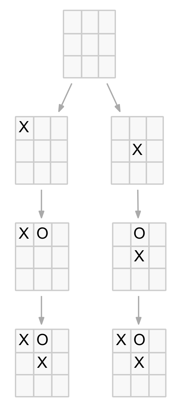
The game can be modelled as a game tree. The starting or root node is the blank board (or grid). This root node has nine child nodes representing the nine possible X-player moves. Each of these nodes has eight child nodes representing the eight possible O-player moves in response to the X-player move. The tree continues in this fashion until either a winning position is reached or the board is full without a winning position being achieved (ie. a draw).

The game tree has 10 levels which will be labelled levels 0 to 9 (technically they should be labelled 1 to 10 but using 0 to 9 works well here as the level number equals the number of moves made at that level). Level 0 will be an empty board (root node) with no moves. Level 1 will be the nine child nodes that represent the first X-move and so on. The diagram below shows a partial game tree.


Partial Game Tree

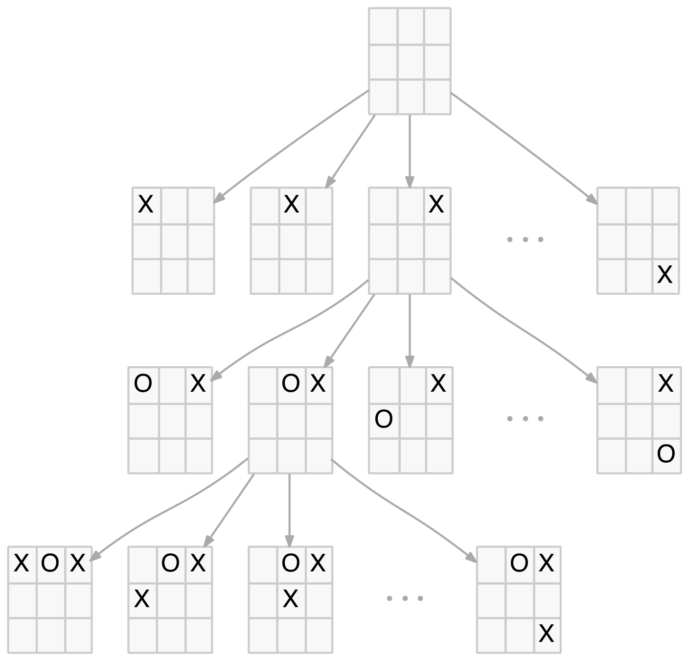
Partial TTT Game Tree

Upper Bounds

It is easy to calculate the maximum size of this tree if we ignore winning positions. This sets an upper bound to the tree size and helps scope the analysis task ahead. Later we will look ways to reduce the size of the tree by:

  • stopping at winning positions
  • identifying duplicate positions
  • accounting for position symmetries
  • considering “forced” moves

It is clear that level 0 has a single empty root node, level 1 has the nine first moves of the X-player. Level 2 will have eight O-player nodes for each of the nine nodes in level 1, or 9×8 nodes in total. Level 3 will have seven nodes for each of the level 2 nodes, or 9x8x7, and so forth until level 9 which will have 9x8x7x6x5x4x3x2x1 nodes. Those familiar with the factorial notation will recognise the level 9 result as 9!. It is easy to see the other levels are just factorial ratios (9!/9!, 9!/8!, 9!/7!, etc).

The following is a summary of the maximum size of the game tree:

Level  Number            Factorial    Total
-------------------------------------------
0      1                   9!/9!          1
1      9                   9!/8!          9
2      9x8                 9!/7!         72
3      9x8x7               9!/6!        504
4      9x8x7x6             9!/5!      3,024
5      9x8x7x6x5           9!/4!     15,120
6      9x8x7x6x5x4         9!/3!     60,480
7      9x8x7x6x5x4x3       9!/2!    181,440
8      9x8x7x6x5x4x3x2     9!/1!    362,880
9      9x8x7x6x5x4x3x2x1   9!/0!    362,880
--------------------------------------------
Total                               986,410

From this we can see any analysis is computationally tractable because at worst there are less than 1 million nodes and the tree depth is a maximum of nine (so recursive analysis is not going to run into stack overflow problems).

Finally we can write some code to determine the tree size if we take into account winning positions. This will prune the tree at each winning node as it will become a leaf or terminal node. We would therefore expect the number of nodes to be reduced from the upper bound after level 5 which is the earliest case that three Xs can occur to make a winning position for the X-player.

Code Approach

To start, we need a representation of the TTT board. A Clojure vector is ideal as its elements can be accessed quickly using a cardinal index. Using a nine element vector to represent the nine cells on the board, its indexes (0-8) will be mapped to the board cells as follows:


Index Mapping

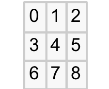
Each vector element, or board cell, will take one of three values represented by the Clojure keywords :x, :o and :e corresponding to an X-player token, an O-player token or an empty cell respectively.

An initially blank board would be represented as [:e :e :e :e :e :e :e :e :e]. As moves are played the :e values will be progressively replaced with :x and :o values.

Winning Positions

To account for winning positions we can simply walk the game tree and test each node for one of two terminal conditions:

  1. Won position for the last player to move
  2. No more empty cells (ie. a draw)

The first thing we need is a couple of helper functions to generate the available moves for a given board and to check for won positions.

(defn gen-moves
  "Return a list of all valid moves on the specified board or nil"
  [board]
  (filter #(= :e (board %)) (range 9)))

(defn win-board?
  "Determine if a board is a win for a given player."
  [board player]
  (let [win-seqs (list [0 1 2] [3 4 5] [6 7 8]    ; Horizontal
                       [0 3 6] [1 4 7] [2 5 8]    ; Vertical
                       [0 4 8] [2 4 6])           ; Diagonal
        win (fn [win-seq] (every? #(= player (board %)) win-seq))]
    (some win win-seqs)))

These functions are fairly straightforward. The first function just returns a sequence of indexes for each empty cell (those containing :e) found on the board or nil if there are none.

The second works its way through a (constant) list of vectors that denote the three indexes that represent the eight (3 x horizontal, 3 x vertical and 2 x diagonal) winning sequences, and checks to see if any hold all three of the given player’s token (:x or :o). If you are new to Clojure you should note that the let form allows you to bind not just values but also functions, and that the win function includes external values within the main function’s scope (‘board’ and ‘player’) in addition to its own ‘win-seq’ argument.

For the initial analysis, the number and type of nodes at each level of the game tree will be determined. To do this the following data structure will be used. It is a map of maps. Each level number is a key of the first map, with its values being a second map of attribute/value pairs. The attributes will be node types and the values will be node counts.

{0 {:attr1 val1, :attr2 val2, ...}
 1 {:attr1 val1, :attr2 val2, ...}
 .
 .
 9 {:attr1 val1, :attr2 val2, ...}}

Returned data structure format

We can now write the main game tree walking function. This is a recursive depth-first function that examines each node and determines whether it is a terminal or internal node. If it is a terminal node (ie. a win or draw) it just returns some details about the node (ie. type and depth). If it is an internal node, it must recursively calls each child node passing updated arguments such as a new board incorporating the specific move for that child. Importantly it must also aggregate the return values for each child, including its own value, and pass them back to its calling parent.

It is also worth noting that we are not walking an existing game tree but rather temporarily constructing it as we go. Indeed only the current node and its immediate ancestors exist at any time (held in the call stack).

(defn ttt-walk
  "Recursively walk the TTT game tree and aggregate results for each node"
  [board last-player next-player level win-board? gen-moves]
  (if (win-board? board last-player)
    {level {last-player 1}}               ; Terminal win node
    (let [moves (gen-moves board)]
      (if (empty? moves)
        {level {:draw 1}}                 ; Terminal draw node
        (reduce (fn [a b] (merge-with #(merge-with + %1 %2) a b))
                {level {:inode 1}}        ; Internal node (inode)
                (for [m moves]
                  (ttt-walk (assoc board m next-player)
                            next-player
                            last-player
                            (inc level)
                            win-board?
                            gen-moves)))))))
(ttt-walk [:e :e :e :e :e :e :e :e :e] :o :x 0 win-board? gen-moves)
;=> (after some reordering for clarity)
{0 {:inode 1},
 1 {:inode 9},
 2 {:inode 72},
 3 {:inode 504},
 4 {:inode 3024},
 5 {:inode 13680, :x 1440},
 6 {:inode 49392, :o 5328},
 7 {:inode 100224, :x 47952},
 8 {:inode 127872, :o 72576},
 9 {:draw 46080, :x 81792}}

The walk function takes the board, the last and next player (clearly only one is required as the other can be deduced but it is simple and clear to use both), the level and the two helper functions it uses (see below). It first checks to see if the board was won by the last player. If so, it returns a fragment of the data structure above with the level, node type and count. Otherwise it gets the available moves and again returns if there are none (ie. a draw) with a similar data structure. Finally, if there are moves, it recursively calls itself for each available move with updated arguments and aggregates the returned results with the reduce function. The reduce function’s reducing function does the heavy lifting combining the data structure fragments returned into one aggregated structure using merge-with (twice) to add together counts from like node types. The initial value of the reduce function is used to include the parent node details.

The code above attempts to be as pure as possible from a functional perspective. In particular, all its inputs are passed as arguments, including functions it calls, rather than using global references, and the returned results are aggregated and passed back up the calling chain. While this approach might be functionally pure it is not particularly pragmatic in this situation. The aggregation of child results is somewhat cumbersome which detracts from the overall intent.

A more straightforward, if less pure, approach is to just update the data structure directly as each node is processed. Clojure was designed with real world state management in mind and it provides several ways to do this safely.

By using a Clojure atom to hold the data structure we can recast the walk function to directly update it using the swap! function. This approach will be continued as the code is enhanced to include further game tree pruning measures. The code is essentially the same only a ‘results’ argument has been added which is a reference to the data structure and, for clarity, the two helper functions are no longer passed as arguments.

One final refinement is the use of a pre-constructed data structure using sorted-maps instead of the default hash-maps. This is purely an aesthetic measure that means the results display in order on my IDE. It would, of course, also be easy to write an output function to display/print the results in any particular order or format. Both the ‘unordered’ and ‘order’ calls are shown below for completeness. The ordered one will be used for all future calls.

(defn ttt-walk
  "Recursively walk the TTT game tree and update results for each node"
  [board last-player next-player level results]
  (if (win-board? board last-player)
    (swap! results update-in [level last-player] (fnil inc 0))  ; Win node
    (let [moves (gen-moves board)]
      (if (empty? moves)
        (swap! results update-in [level :draw] (fnil inc 0))    ; Draw node
        (do
          (swap! results update-in [level :inode] (fnil inc 0)) ; Internal node
          (doseq [m moves]
            (ttt-walk (assoc board m next-player)
                      next-player
                      last-player
                      (inc level)
                      results)))))))
(let [results (atom {})]
  (ttt-walk [:e :e :e :e :e :e :e :e :e] :o :x 0 results)
  @results)
;
; By setting up an empty result structure using 'sorted-maps' instead
; of the default (unsorted) 'hash-map' the output is correctly ordered.
;
(let [resmap (into (sorted-map) (for [n (range 10)] [n (sorted-map)]))
      results (atom resmap)]
  (ttt-walk [:e :e :e :e :e :e :e :e :e] :o :x 0 results)
  @results)
;=>
{0 {:inode 1},
 1 {:inode 9},
 2 {:inode 72},
 3 {:inode 504},
 4 {:inode 3024},
 5 {:inode 13680, :x 1440},
 6 {:inode 49392, :o 5328},
 7 {:inode 100224, :x 47952},
 8 {:inode 127872, :o 72576},
 9 {:draw 46080, :x 81792}}

Gratifyingly the results from both versions of the walk function are identical and are in line with what would be expected from the initial upper bound calculations. For the first four levels, where no winning positions can occur the node counts exactly match the calculated ones. At the fifth level, we see the first X-player winning position counts but note the sum of these and the internal nodes still equals the calculated count as expected. From there on, the actual node counts reduce compared to the calculated ones as the winning nodes no longer have children. Also, as expected, the X-player wins occur on the odd levels, while the O-player wins occur on the even levels.

The table below summarises these results. This table will be used to track our progress as we implement later pruning measures. Note a drawn node (marked :draw in the code results) is the same as a level 9 internal node (:inode). So for brevity, in the table, drawn nodes are shown on the ‘Internal’ node line at level 9 rather than on a separate line of their own.

Node Level 0 1 2 3 4 5 6 7 8 9 Total
Upper Bound 1 9 72 504 3,024 15,120 60,480 181,440 362,880 362,880 986,410
Actual after accounting for winning nodes
Internal 1 9 72 504 3,024 13,680 49,392 100,224 127,872 46,080 340,858
X-wins 1,440 47,952 81,792 131,184
O-wins 5,328 72,576 77,904
Total 1 9 72 504 3,024 15,120 54,720 148,176 200,448 127,872 549,946

As the table shows, by taking account of winning positions the size of the game tree is reduced by almost a half. Are there other ways we can prune the tree?

Duplicated Positions

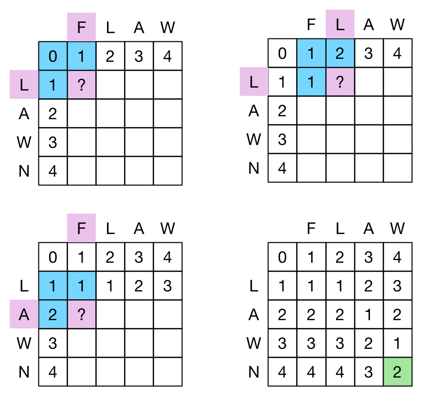
A little thought leads to the realisation that the same position can be reached by different combinations of the same moves. This means identical positions will occur in different branches of the tree. A simple example is shown below.


Duplicate Node Example

Duplicated node example

Not only are these positions duplicated but all their descendants are also duplicated in later levels. The degree of duplication can be calculated based on the number of moves made by each player. For example, in a position with three Xs and two Os, the first X could be played in any of three places, the second X in any of the two remaining places and the third in the one remaining place which is 3x2x1 or 3! ways. Similarly the first O can be in either of two positions and then in the one remaining position which is 2×1 or 2! ways. So in total there are 3!2! = 12 ways that position could have been reached. In general, if a position has n Xs and m Os then there are n!m! duplicates of that position. If we recalculate the upper bound discounting for duplicate nodes we get a significant reduction in the game tree size as shown in the updated table below:

                                             Duplication  De-duplicated
Level  Number            Factorial    Total    Factor         Total
-----------------------------------------------------------------------
0      1                   9!/9!          1   0!x0!=1            1
1      9                   9!/8!          9   1!x0!=1            9
2      9x8                 9!/7!         72   1!x1!=1           72
3      9x8x7               9!/6!        504   2!x1!=2          252
4      9x8x7x6             9!/5!      3,024   2!x2!=4          756
5      9x8x7x6x5           9!/4!     15,120   3!x2!=12        1260
6      9x8x7x6x5x4         9!/3!     60,480   3!x3!=36        1680
7      9x8x7x6x5x4x3       9!/2!    181,440   4!x3!=144       1260
8      9x8x7x6x5x4x3x2     9!/1!    362,880   4!x4!=576        630
9      9x8x7x6x5x4x3x2x1   9!/0!    362,880   5!x4!=2880       126
-----------------------------------------------------------------------
Total                               986,410                   6046

The ‘De-duplicated Total’ column is just the original ‘Total’ column divided by the ‘Duplication Factor’.

The tree walking code above can be readily modified to check for duplicates by maintaining a set of board positions as the tree is walked and checking each new node for membership of that set. The modified code below has the main changes highlighted. Note a new argument ‘dups’ is introduced to hold known boards (ie. those already visited).

(defn ttt-walk
  "Recursively walk the TTT game tree and update results for each node"
  [board last-player next-player level dups results]
  (if (contains? @dups board)
    (swap! results update-in [level :dup] (fnil inc 0))  ; Duplicate node
    (do
      (swap! dups conj board)
      (if (win-board? board last-player)
        (swap! results update-in [level last-player] (fnil inc 0))  ; Win node
        (let [moves (gen-moves board)]
          (if (empty? moves)
            (swap! results update-in [level :draw] (fnil inc 0))    ; Draw node
            (do
              (swap! results update-in [level :inode] (fnil inc 0)) ; Internal node
              (doseq [m moves]
                (ttt-walk (assoc board m next-player)
                          next-player
                          last-player
                          (inc level)
                          dups
                          results)))))))))
(let [resmap (into (sorted-map) (for [n (range 10)] [n (sorted-map)]))
      results (atom resmap)
      dups (atom #{})]
  (ttt-walk [:e :e :e :e :e :e :e :e :e] :o :x 0 dups results)
  @results)
;=>
{0 {:inode 1},
 1 {:inode 9},
 2 {:inode 72},
 3 {:dup 252, :inode 252},
 4 {:dup 756, :inode 756},
 5 {:dup 2520, :inode 1140, :x 120},
 6 {:dup 3040, :inode 1372, :o 148},
 7 {:dup 2976, :inode 696, :x 444},
 8 {:dup 1002, :inode 222, :o 168},
 9 {:draw 16, :dup 144, :x 62}}

As shown by the updated tracking table below, these results align well with the new de-duplicated upper bound. They match perfectly up to level 5 when winning nodes start to prune the tree and the node counts drop away as in the earlier example. The large reduction in the size of the tree is also encouraging as it hints at the underlying simplicity of the game.

Node Level 0 1 2 3 4 5 6 7 8 9 Total
Upper Bound 1 9 72 504 3,024 15,120 60,480 181,440 362,880 362,880 986,410
Actual after accounting for winning nodes
Internal 1 9 72 504 3,024 13,680 49,392 100,224 127,872 46,080 340,858
X-wins 1,440 47,952 81,792 131,184
O-wins 5,328 72,576 77,904
Total 1 9 72 504 3,024 15,120 54,720 148,176 200,448 127,872 549,946
After accounting for duplicate nodes
Upper Bound 1 9 72 252 756 1,260 1,680 1,260 630 126 6,046
Actual after accounting for duplicate and winning nodes
Internal 1 9 72 252 756 1,140 1,372 696 222 16 4,536
X-wins 120 444 62 626
O-wins 148 168 316
Total 1 9 72 252 756 1,260 1,520 1,140 390 78 5,478

Symmetric Positions

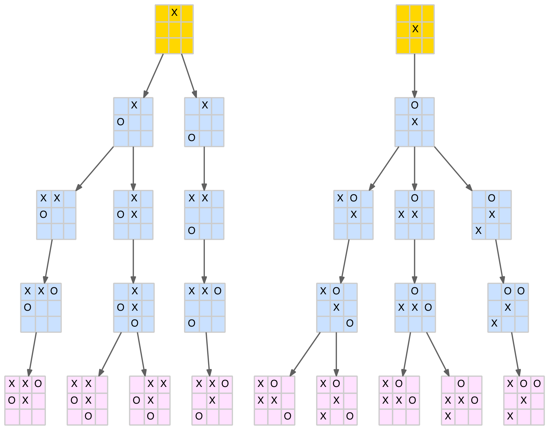
The next stage in tree pruning is to account for position symmetries. It is fairly obvious that although there are nine first X-player moves, only three are distinct (a corner, an edge or the centre). The rest are just rotations or reflections of these three. The same holds for the O-player responses to these three moves. There are only five, five and two, respectively, distinct responses as shown in the diagram below.


First two moves excluding symmetrical positions

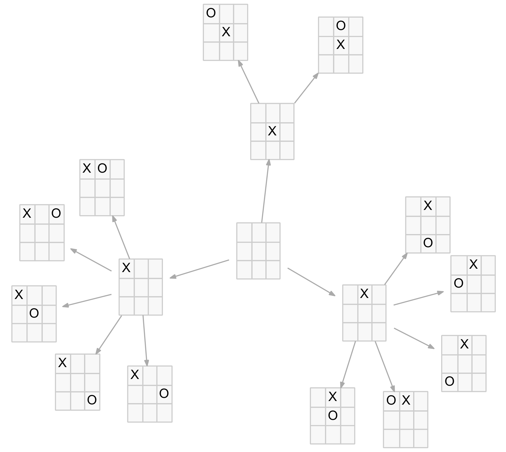
Distinct positions after two moves

This means instead of the original 9×8=72 nodes at level 2 in the game tree there are actually only 12 distinct nodes. Similar symmetries exist at other levels. A little experimentation (or theory for those with linear transformation skills) shows there are seven symmetries involved: 3 rotations (90, 180 and 270 degrees) and 4 reflections (horizontally, vertically and along the two diagonals).

For some positions, not all of these symmetries yield unique new positions (ie. after a transformation the new position is either identical to the original or to one of the other transformations). But many positions do result in seven unique new positions, one example is shown below.


Seven symmetries

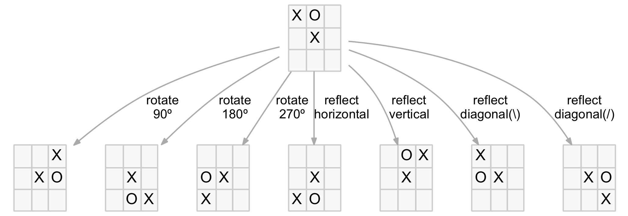
Seven symmetric transformations

To account for symmetries, a new helper function is required that will return a set of boards that are symmetries of the specified board. These boards can then be bypassed in the same way as duplicates. Note that duplicates and symmetries are orthogonal (ie. they don’t overlap) so there is no interference between them that might affect node counts or the order in which they are tested/excluded.

(defn board-symmetries
  "Return a set of all symmetric boards based on rotations and
  reflections of the specified board."
  [board]
  (let [transforms
        [[6 3 0 7 4 1 8 5 2]    ; Rotation of 90 degrees
         [8 7 6 5 4 3 2 1 0]    ; Rotation of 180 degrees
         [2 5 8 1 4 7 0 3 6]    ; Rotation of 270 degrees
         [6 7 8 3 4 5 0 1 2]    ; Horizontal reflection about 3 4 5
         [2 1 0 5 4 3 8 7 6]    ; Vertical reflection about 1 4 7
         [0 3 6 1 4 7 2 5 8]    ; Diagonal reflection about 0 4 8
         [8 5 2 7 4 1 6 3 0]]]  ; Diagonal reflection about 2 4 6
    (disj (set (for [t transforms] (vec (map board t)))) board)))

The function above uses vectors to hold index mappings of each transformation (rotations and reflections) which it applies to the specified board to produce seven new boards. These are combined into a set which will eliminate any identical boards and disj is used to remove the original board if it happened to be generated by one of the transformations.

With duplicates we just added (conj) each new board as it was processed for later checking. For symmetries we need to add all the symmetric boards that arise so we use the union function to maintain a set of all boards that are known to be symmetries of processed nodes.

The previous tree walking code has been modified to track and bypass symmetric nodes. The main changes are highlighted. Note a new argument ‘syms’ is introduced to hold symmetric boards.

(defn ttt-walk
  "Recursively walk the TTT game tree and update results for each node"
  [board last-player next-player level dups syms results]
  (cond
    (contains? @dups board)
      (swap! results update-in [level :dup] (fnil inc 0))  ; Duplicate node
    (contains? @syms board)
      (swap! results update-in [level :sym] (fnil inc 0))  ; Symmetric node
    :else
      (do
        (swap! dups conj board)
        (swap! syms clojure.set/union (board-symmetries board))
        (if (win-board? board last-player)
          (swap! results update-in [level last-player] (fnil inc 0))  ; Win node
          (let [moves (gen-moves board)]
            (if (empty? moves)
              (swap! results update-in [level :draw] (fnil inc 0))    ; Draw node
              (do
                (swap! results update-in [level :inode] (fnil inc 0)) ; Internal node
                (doseq [m moves]
                  (ttt-walk (assoc board m next-player)
                            next-player
                            last-player
                            (inc level)
                            dups
                            syms
                            results)))))))))
(let [resmap (into (sorted-map) (for [n (range 10)] [n (sorted-map)]))
      results (atom resmap)
      dups (atom #{})
      syms (atom #{})]
  (ttt-walk [:e :e :e :e :e :e :e :e :e] :o :x 0 dups syms results)
  @results)
;=>
{0 {:inode 1},
 1 {:inode 3, :sym 6},
 2 {:inode 12, :sym 12},
 3 {:dup 3, :inode 38, :sym 43},
 4 {:dup 44, :inode 108, :sym 76},
 5 {:dup 161, :inode 153, :sym 205, :x 21},
 6 {:dup 225, :inode 183, :o 21, :sym 183},
 7 {:dup 220, :inode 95, :sym 176, :x 58},
 8 {:dup 82, :inode 34, :o 23, :sym 51},
 9 {:draw 3, :dup 11, :sym 8, :x 12}}

Again these results look consistent with our expectations. The counts for level 1 and 2 agree with the 3 and 12 node counts identified in the diagram above, and the overall node counts have shrunk again at all levels.

As shown by the following updated tracking table we are now down to a game tree of just 765 nodes, a big reduction from the half million plus we started with.

Node Level 0 1 2 3 4 5 6 7 8 9 Total
Upper Bound 1 9 72 504 3,024 15,120 60,480 181,440 362,880 362,880 986,410
Actual after accounting for winning nodes
Internal 1 9 72 504 3,024 13,680 49,392 100,224 127,872 46,080 340,858
X-wins 1,440 47,952 81,792 131,184
O-wins 5,328 72,576 77,904
Total 1 9 72 504 3,024 15,120 54,720 148,176 200,448 127,872 549,946
After accounting for duplicate nodes
Upper Bound 1 9 72 252 756 1,260 1,680 1,260 630 126 6,046
Actual after accounting for duplicate and winning nodes
Internal 1 9 72 252 756 1,140 1,372 696 222 16 4,536
X-wins 120 444 62 626
O-wins 148 168 316
Total 1 9 72 252 756 1,260 1,520 1,140 390 78 5,478
Actual after accounting for symmetric, duplicate and winning nodes
Internal 1 3 12 38 108 153 183 95 34 3 630
X-wins 21 58 12 91
O-wins 21 23 44
Total 1 3 12 38 108 174 204 153 57 15 765

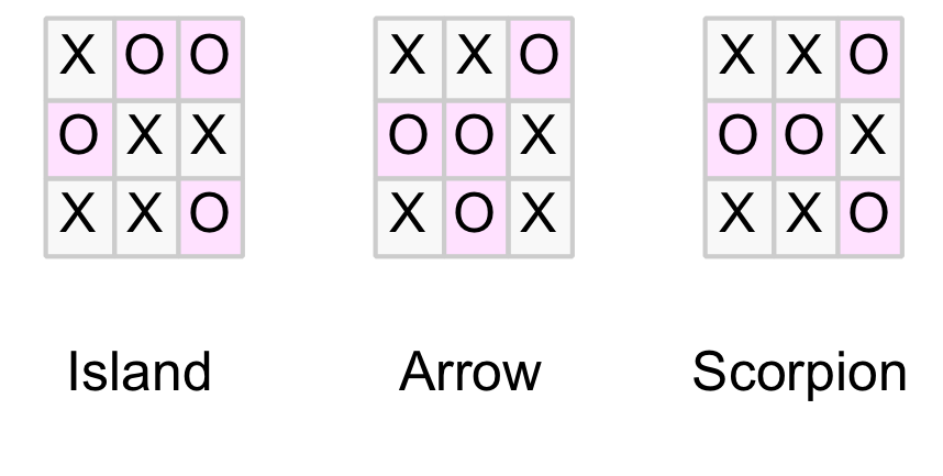
One interesting result is that there are only three distinct drawn boards (shown below). As they can occur in different orientations it is easier to recognise them as patterns. The Os are highlighted below to emphasis the shape and some euphemistic names are attached (although the reader may have better suggestions).


Drawn positions

The three patterns for all drawn boards

Looking at it another way, for a position to be a draw, the four O-tokens must cover all the winning sequences and must not form a winning sequence themselves. So at least one O-token must be in each row, column and diagonal. This significantly limits the number of combinations. The code below does a quick check of all the ways four tokens can be placed on a board so that they cover each of the eight winning sequences but don’t create a winning sequence themselves. (Please note this code is optimised for clarity, not performance, as it is a one-off but it still runs in under 0.5 seconds on my laptop.)

(def win-seqs [[0 1 2] [3 4 5] [6 7 8]  ; Horizontal wins
               [0 3 6] [1 4 7] [2 5 8]  ; Vertical wins
               [0 4 8] [2 4 6]])        ; Diagonal wins

(for [a (range 9) b (range 9) c (range 9) d (range 9)
      :let [x (set [a b c d])]
      :when (and
              (< a b c d)
              (every? #(some x %) win-seqs)
              (every? #(not-every? x %) win-seqs))]
  [a b c d])
;=>
([0 1 5 6] [0 2 3 7] [0 2 4 7] [0 2 5 7]
 [0 4 5 6] [0 4 5 7] [0 5 6 7] [1 2 3 8]
 [1 3 4 8] [1 3 6 8] [1 4 5 6] [1 4 6 8]
 [1 5 6 8] [2 3 4 7] [2 3 4 8] [2 3 7 8])

The reader can confirm that the resulting 16 indexes represent 4 x Arrow, 4 x Scorpion, and 8 x Island patterns as would be expected when symmetries are taken into account (note the tracking table shows 16 drawn boards before symmetries were excluded).

It is a testament to the power of Clojure (and similar modern languages) that this check can be programmed in a few lines of code (technically two). Not only is the code concise, it is also ‘safe’ in the sense that edge-cases, boundary conditions, etc. are all abstracted away.

Forcing Moves

One final refinement which leads into the second part of this blog – covering player strategy – is that most players are able to spot a winning sequence if it is available and also a blocking move should the opponent be about to win (ie. has two-in-a-row). We can further prune the tree by assuming a player will always:

  1. make a winning move if one is available (and forgo all other moves)
  2. make a blocking move if the opponent threatens to win on the next move (ie. the opponent has two-in-a-row)

A straightforward way to achieve this is to modify the move generating function to check the above conditions, and if found, to return only a single move (ie. either the winning or blocking move). If the conditions don’t apply then return the list of all valid moves as before.

The modified function (now called gen-moves-forced) is shown below. Note ‘next-player’ and ‘last-player’ variables have been abbreviated to ‘next-p’ and ‘last-p’ so the code fits better on the limited blog real estate – not a practice I would normally encourage :).

(defn gen-moves-forced
  "Return a restricted list of moves based on these priorities:
  1. Make a winning move if one exists
  2. Block the opponent from winning
  3. Otherwise - make any move (ie. return all valid moves)"
  [board last-p next-p]
  (let [moves (filter #(= :e (board %)) (range 9))
        wins (filter #(win-board? (assoc board % next-p) next-p) moves)
        blocks (filter #(win-board? (assoc board % last-p) last-p) moves)]
    (cond
      (not-empty wins) (list (first wins))
      (not-empty blocks) (list (first blocks))
      :else moves)))

The code above initially generates all moves as before (‘moves’). Then for each move determines which ones (if any) create a winning board for the next-player (‘wins’) and similarly winning options for the last-player (‘blocks’). If there is a win or wins for the next-player, return one. If there is no win but a block or blocks, return one. Otherwise return all available moves as before.

Now the walk code can be re-run using the modified move generation function (highlighted below).

(defn ttt-walk
  "Recursively walk the TTT game tree and update results for each node"
  [board last-player next-player level dups syms results]
  (cond
    (contains? @dups board)
      (swap! results update-in [level :dup] (fnil inc 0))  ; Duplicate node
    (contains? @syms board)
      (swap! results update-in [level :sym] (fnil inc 0))  ; Symmetric node
    :else
      (do
        (swap! dups conj board)
        (swap! syms clojure.set/union (board-symmetries board))
        (if (win-board? board last-player)
          (swap! results update-in [level last-player] (fnil inc 0))  ; Win node
          (let [moves (gen-moves-forced board last-player next-player)]
            (if (empty? moves)
              (swap! results update-in [level :draw] (fnil inc 0))    ; Draw node
              (do
                (swap! results update-in [level :inode] (fnil inc 0)) ; Internal node
                (doseq [m moves]
                  (ttt-walk (assoc board m next-player)
                            next-player
                            last-player
                            (inc level)
                            dups
                            syms
                            results)))))))))
(let [resmap (into (sorted-map) (for [n (range 10)] [n (sorted-map)]))
      results (atom resmap)
      dups (atom #{})
      syms (atom #{})]
  (ttt-walk [:e :e :e :e :e :e :e :e :e] :o :x 0 dups syms results)
  @results)
;=>
{0 {:inode 1},
 1 {:inode 3, :sym 6},
 2 {:inode 12, :sym 12},
 3 {:dup 3, :inode 38, :sym 43},
 4 {:dup 27, :inode 54, :sym 47},
 5 {:dup 21, :inode 88, :sym 41},
 6 {:dup 28, :inode 83, :sym 28},
 7 {:dup 18, :inode 47, :sym 25, :x 25},
 8 {:dup 12, :inode 18, :o 11, :sym 11},
 9 {:draw 3, :dup 4, :sym 5, :x 6}}

We see a further reduction in the game tree size with the inclusion of forced moves. The game tree is now down to just 389 nodes! The updated tracking table below.

Node Level 0 1 2 3 4 5 6 7 8 9 Total
Upper Bound 1 9 72 504 3,024 15,120 60,480 181,440 362,880 362,880 986,410
Actual after accounting for winning nodes
Internal 1 9 72 504 3,024 13,680 49,392 100,224 127,872 46,080 340,858
X-wins 1,440 47,952 81,792 131,184
O-wins 5,328 72,576 77,904
Total 1 9 72 504 3,024 15,120 54,720 148,176 200,448 127,872 549,946
After accounting for duplicate nodes
Upper Bound 1 9 72 252 756 1,260 1,680 1,260 630 126 6,046
Actual after accounting for duplicate and winning nodes
Internal 1 9 72 252 756 1,140 1,372 696 222 16 4,536
X-wins 120 444 62 626
O-wins 148 168 316
Total 1 9 72 252 756 1,260 1,520 1,140 390 78 5,478
Actual after accounting for symmetric, duplicate and winning nodes
Internal 1 3 12 38 108 153 183 95 34 3 630
X-wins 21 58 12 91
O-wins 21 23 44
Total 1 3 12 38 108 174 204 153 57 15 765
Actual after accounting for forced, symmetric, duplicate and winning nodes
Internal 1 3 12 38 54 88 83 47 18 3 347
X-wins 25 6 31
O-wins 11 11
Total 1 3 12 38 54 88 83 72 29 9 389

There are two noteworthy changes:

  1. the X-wins at level 5 and O-wins at level 6 have gone
  2. despite the fact that a player now always blocks an opponent’s winning threat (ie. two-in-a-row) there are still won positions for both the X-player and the O-player

The first point makes sense as the easy wins (through careless defending) no longer occur as the opponent will now always block a two-in-a-row threat.

But what is going on with the second point? Is the code wrong?

No! In fact, it reveals about the only interesting tactical feature of the game. It is possible to create a position with two winning threats (ie. 2 x two-in-a-row) at the same time. This is called a fork. As the opponent can only block one, a player that can achieve a forked position is guaranteed to win.

Below are some examples of forked positions with the two threats highlighted. The first two show the O-player to move and are winning for the X-player. The last one shows the X-player to move and is winning for the O-player.


Fork positions

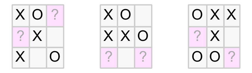
Fork position examples

To understand the number and level of forked positions we need another helper function that tests for these positions. The tree walking code can then be modified to record the forked position details. Remember a forked node is still an internal node, so we would expect the previous :inode count to split between non-forked (:inode) internal nodes and forked (:fork) internal nodes.

The code below shows the helper function, modified walk code (highlighted) and results.

(defn fork-board?
  "Return true if it is a winning 'fork' board for the specified player.
  That is last-player has two winning moves AND next-player has none"
  [board last-p next-p]
  (let [moves (filter #(= :e (board %)) (range 9))
        next-wins (filter #(win-board? (assoc board % next-p) next-p) moves)
        last-wins (filter #(win-board? (assoc board % last-p) last-p) moves)]
    (and (= (count last-wins) 2) (zero? (count next-wins)))))
(defn ttt-walk
  "Recursively walk the TTT game tree and update results for each node"
  [board last-player next-player level dups syms results]
  (cond
    (contains? @dups board)
      (swap! results update-in [level :dup] (fnil inc 0))  ; Duplicate node
    (contains? @syms board)
      (swap! results update-in [level :sym] (fnil inc 0))  ; Symmetric node
    :else
      (do
        (swap! dups conj board)
        (swap! syms clojure.set/union (board-symmetries board))
        (if (win-board? board last-player)
          (swap! results update-in [level last-player] (fnil inc 0))  ; Win node
          (let [moves (gen-moves-forced board last-player next-player)]
            (if (empty? moves)
              (swap! results update-in [level :draw] (fnil inc 0))    ; Draw node
              (do
                (if (fork-board? board last-player next-player)
                  (swap! results update-in [level :fork] (fnil inc 0))   ; Internal fork
                  (swap! results update-in [level :inode] (fnil inc 0))) ; Internal node
                (doseq [m moves]
                  (ttt-walk (assoc board m next-player)
                            next-player
                            last-player
                            (inc level)
                            dups
                            syms
                            results)))))))))
(let [resmap (into (sorted-map) (for [n (range 10)] [n (sorted-map)]))
      results (atom resmap)
      dups (atom #{})
      syms (atom #{})]
  (ttt-walk [:e :e :e :e :e :e :e :e :e] :o :x 0 dups syms results)
  @results)
;=>
{0 {:inode 1}
 1 {:inode 3, :sym 6}
 2 {:inode 12, :sym 12}
 3 {:dup 3, :inode 38, :sym 43}
 4 {:dup 27, :inode 54, :sym 47}
 5 {:dup 21, :fork 36, :inode 52, :sym 41}
 6 {:dup 28, :fork 14, :inode 69, :sym 28}
 7 {:dup 18, :fork 9, :inode 38, :sym 25, :x 25}
 8 {:dup 12, :inode 18, :o 11, :sym 11}
 9 {:draw 3, :dup 4, :sym 5, :x 6}}

These results show forked positions start at level 5 (3 x Xs and 2 x Os) which is expected as at least three Xs are required to form a fork. Also the sum of the forked and non-forked nodes equals the previous internal node counts. There is also a reasonably large number of forked positions suggesting that forks are a significant tactical component of the game.

Visualisation

Until now we have mainly dealt with the size and shape of the TTT game tree. However, as we have managed to prune it down to a relatively small number of nodes, it is possible to display it, or part of it, directly. Using the fantastic Graphviz and the convenient Clojure library dorothy that greatly simplifies creating Graphviz configurations from Clojure, it is relatively straightforward to create a visual representation of the game tree.

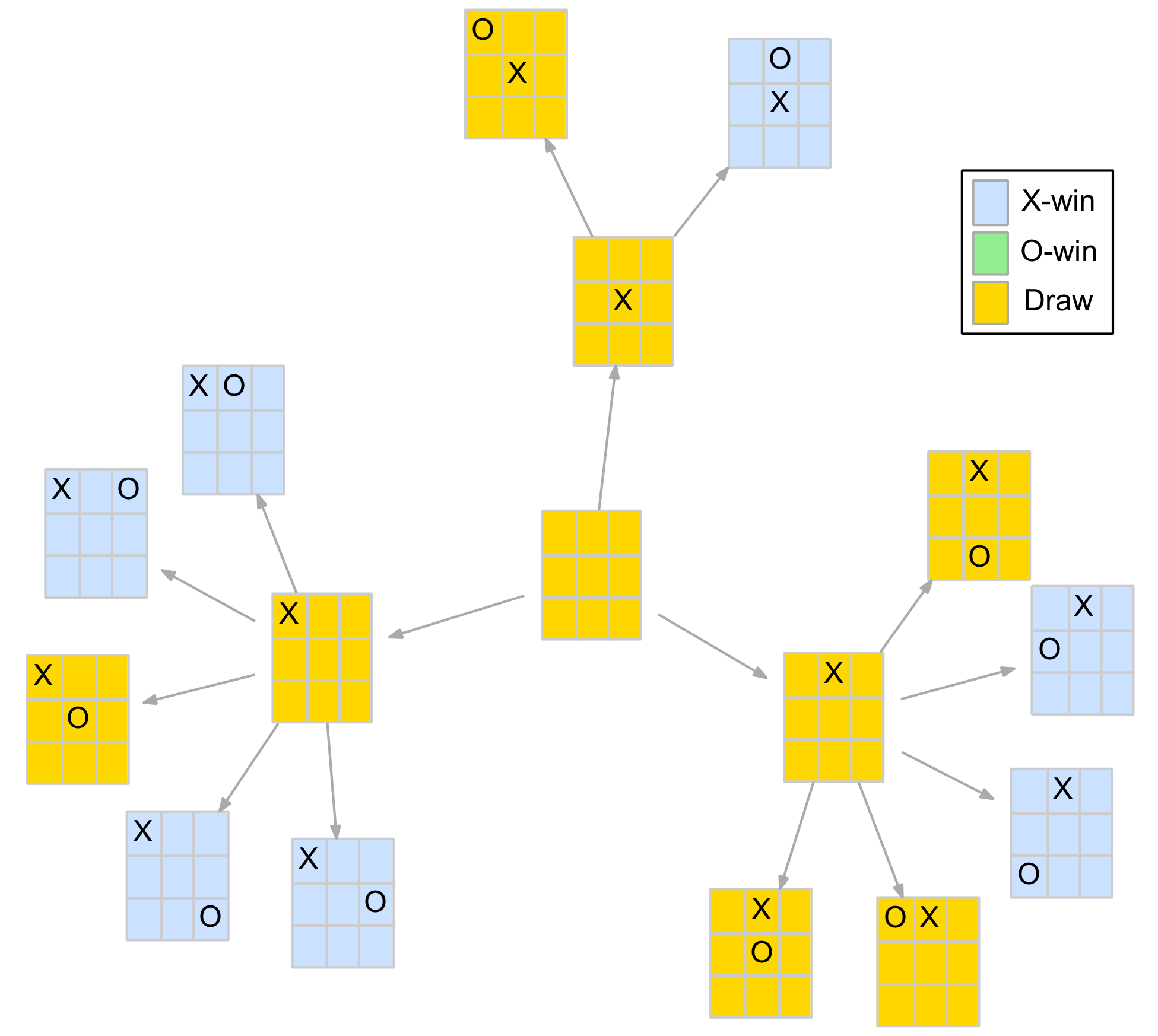
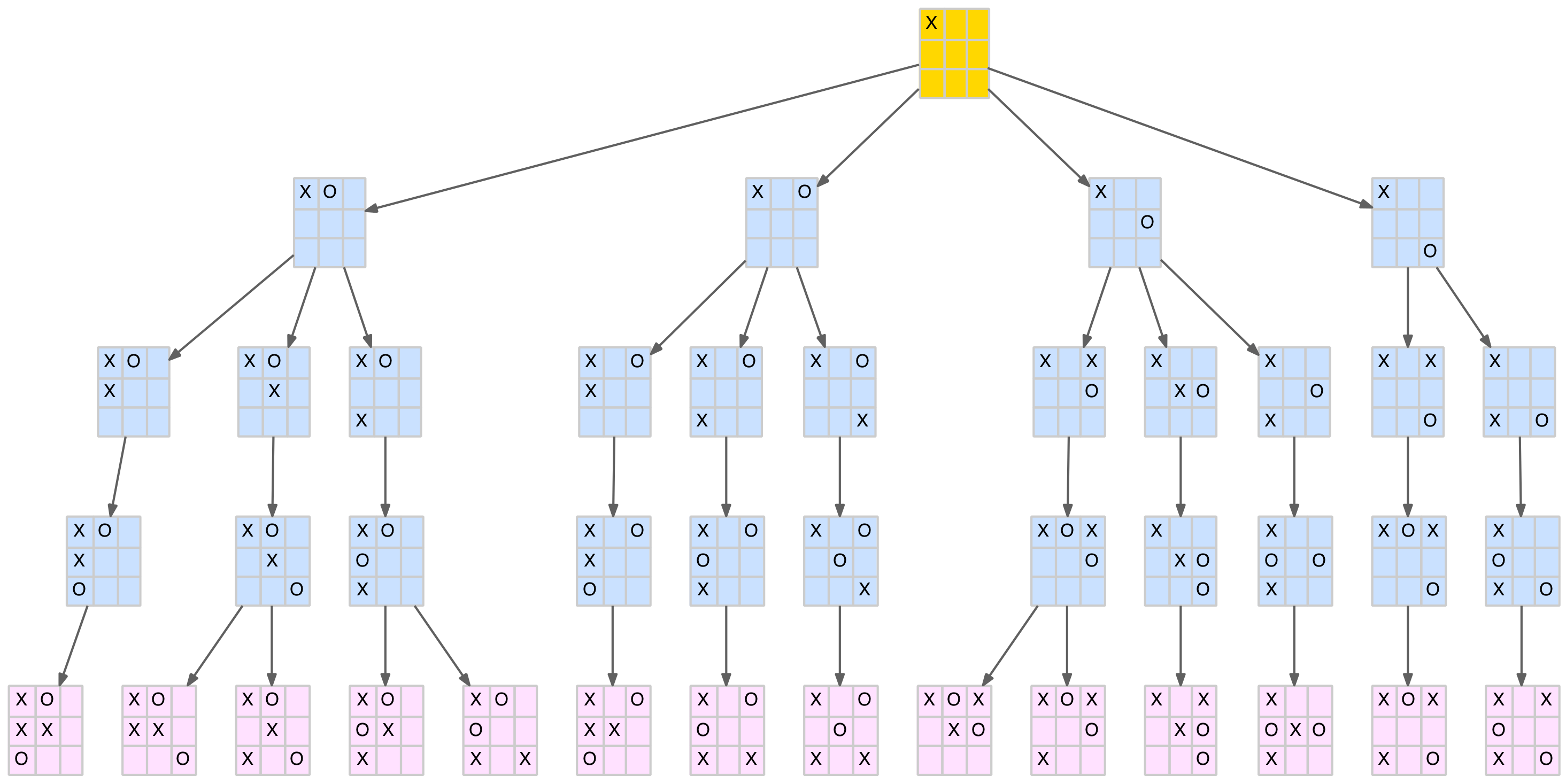
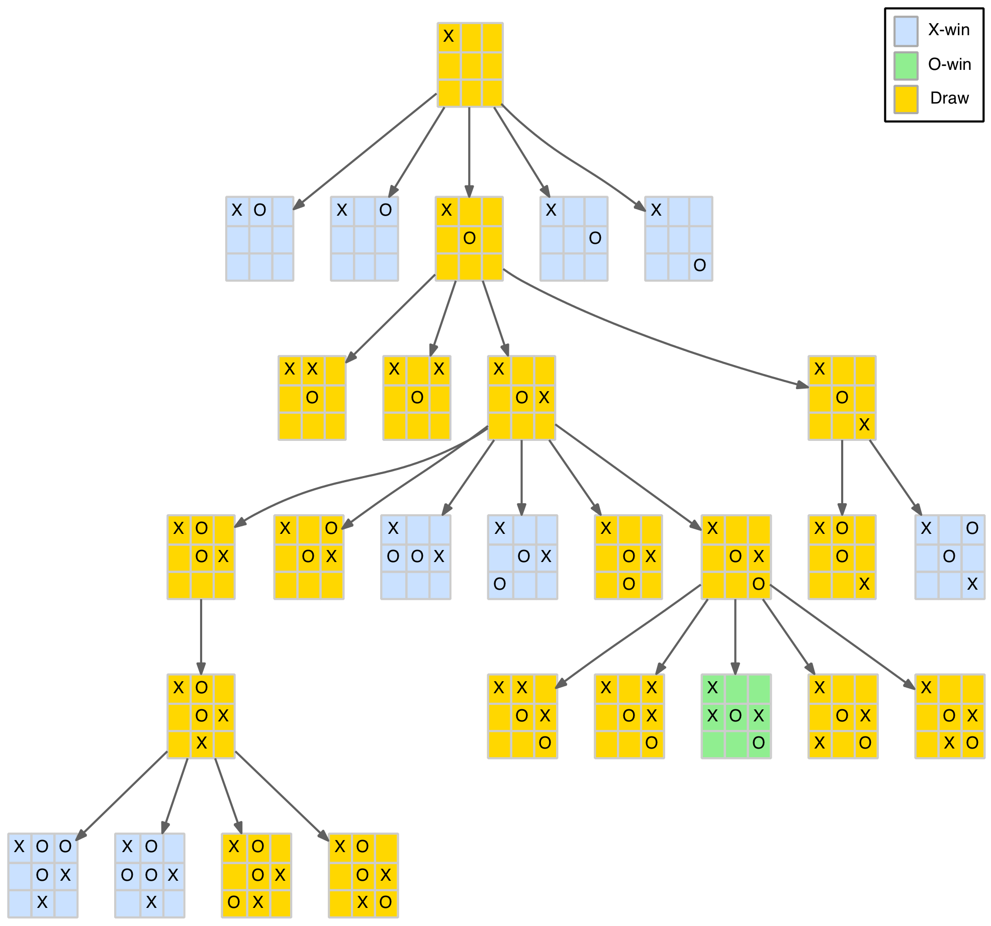
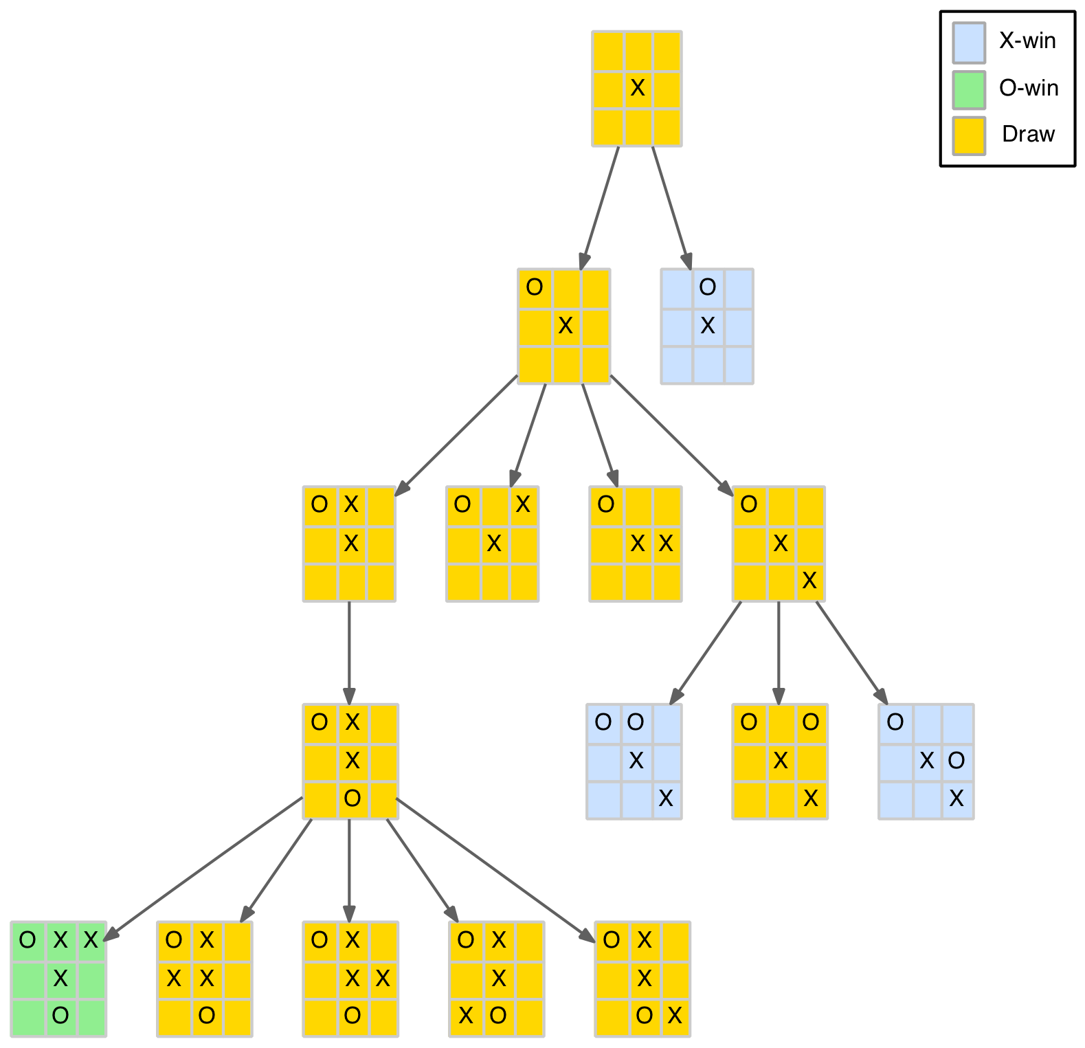
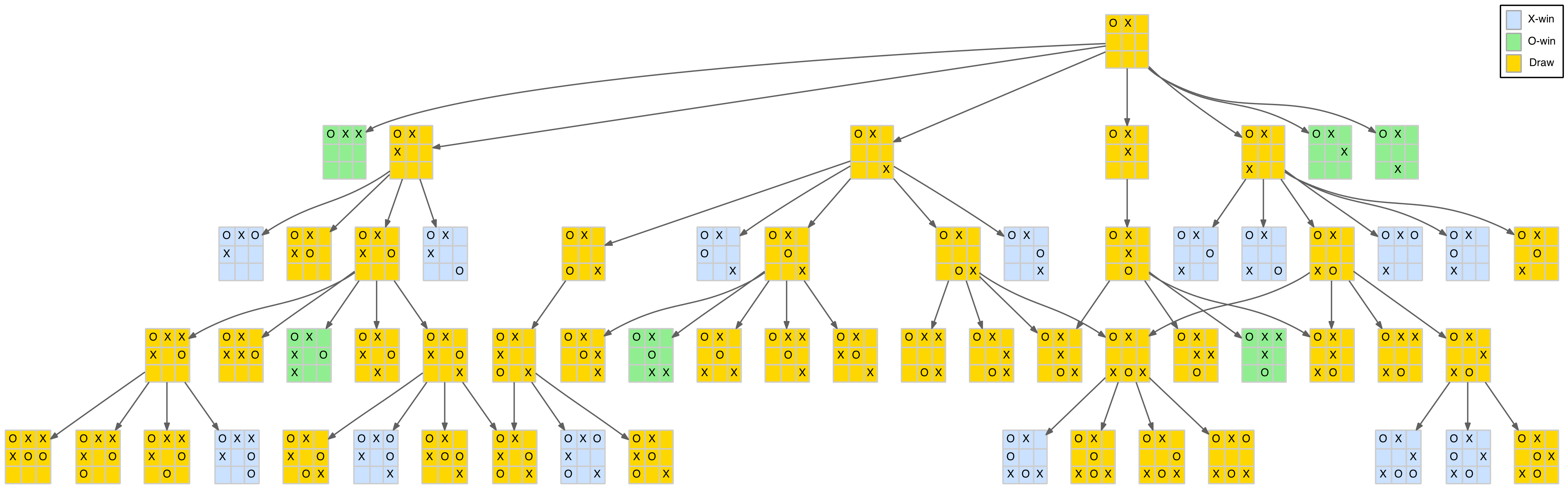
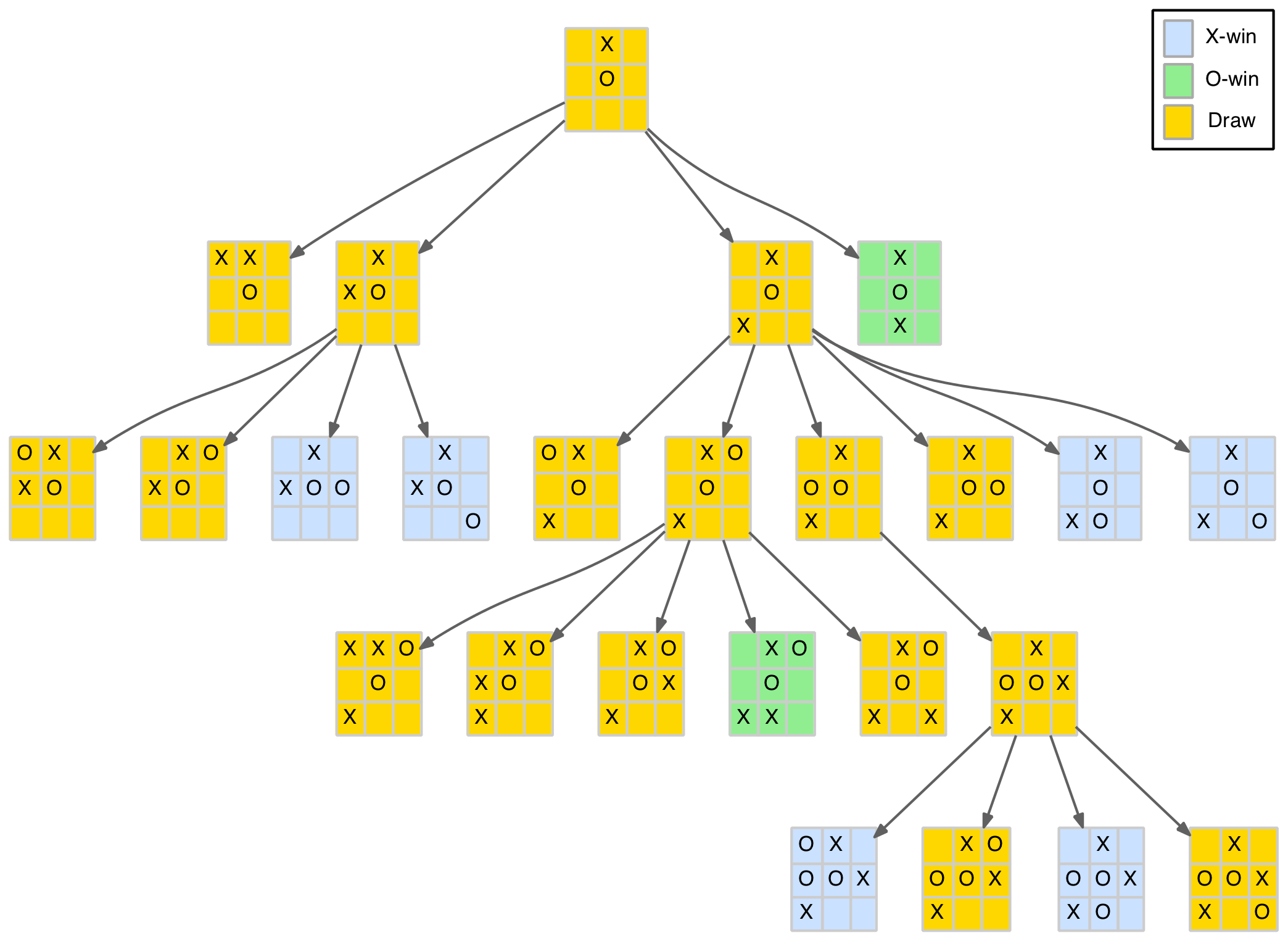
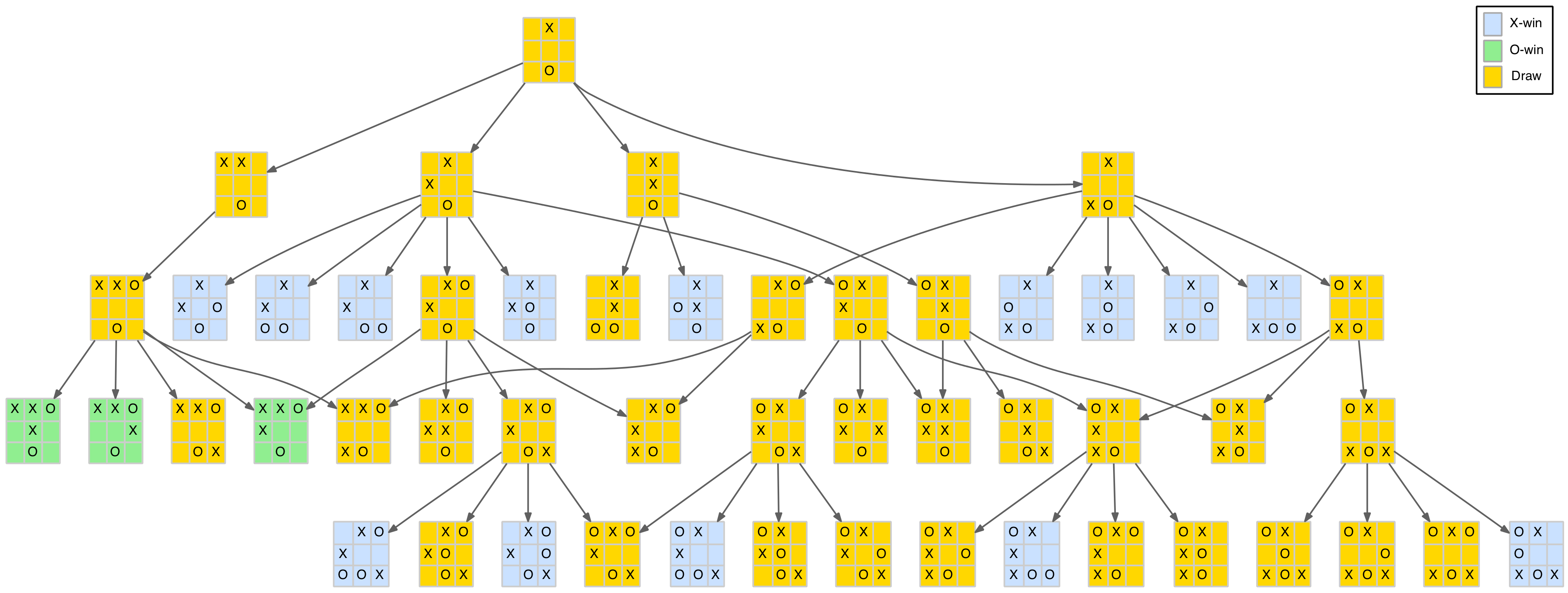
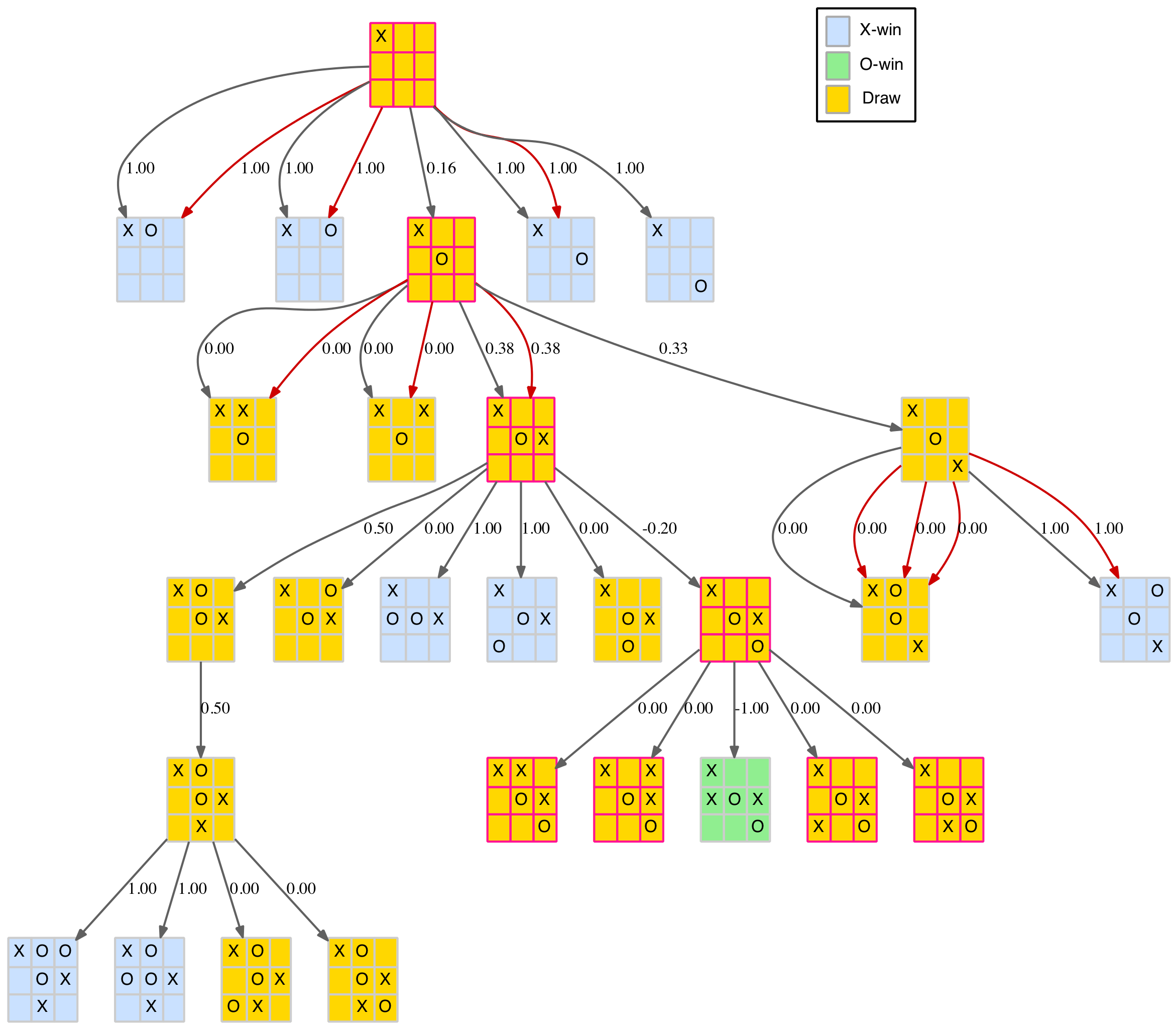
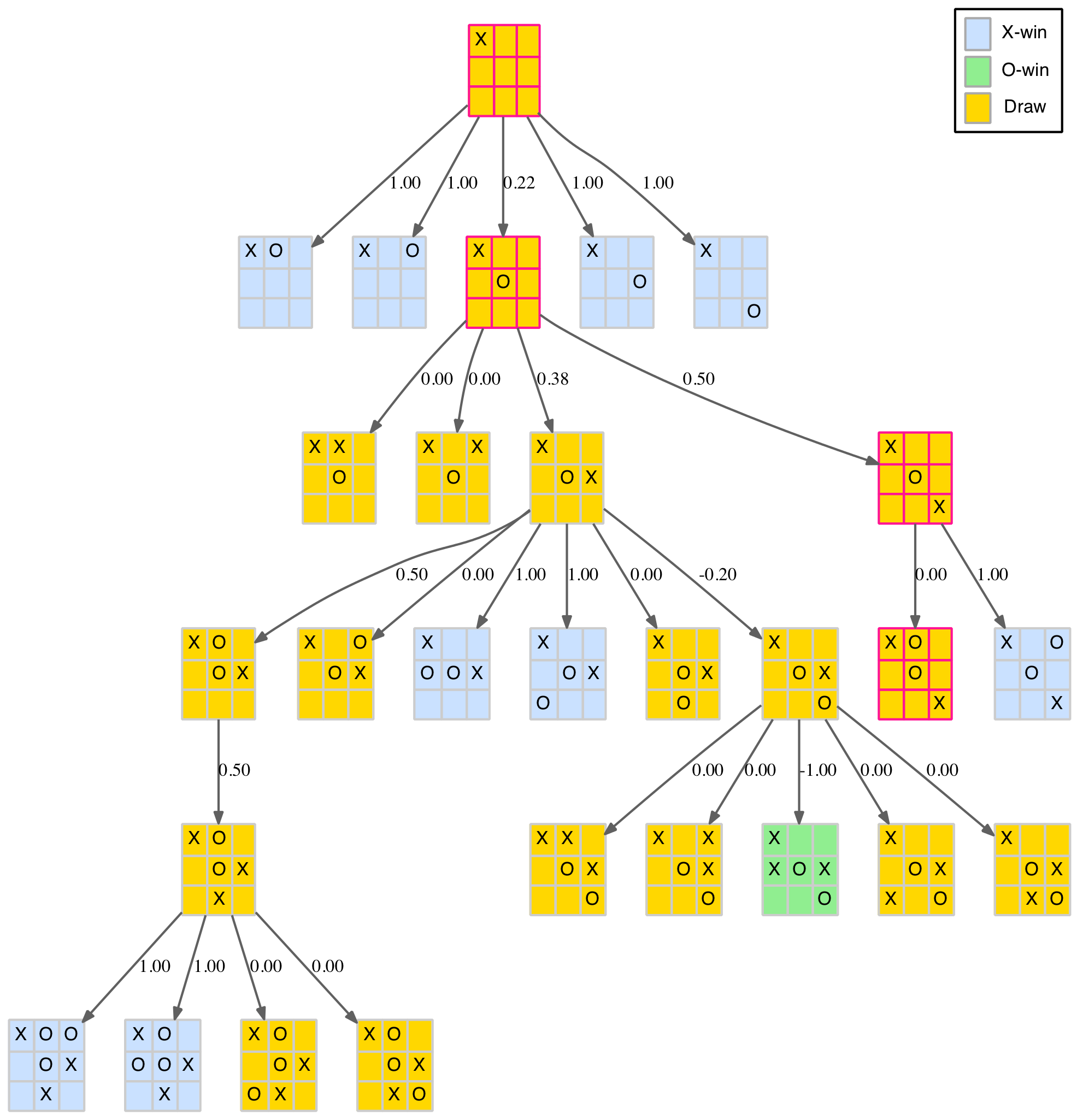
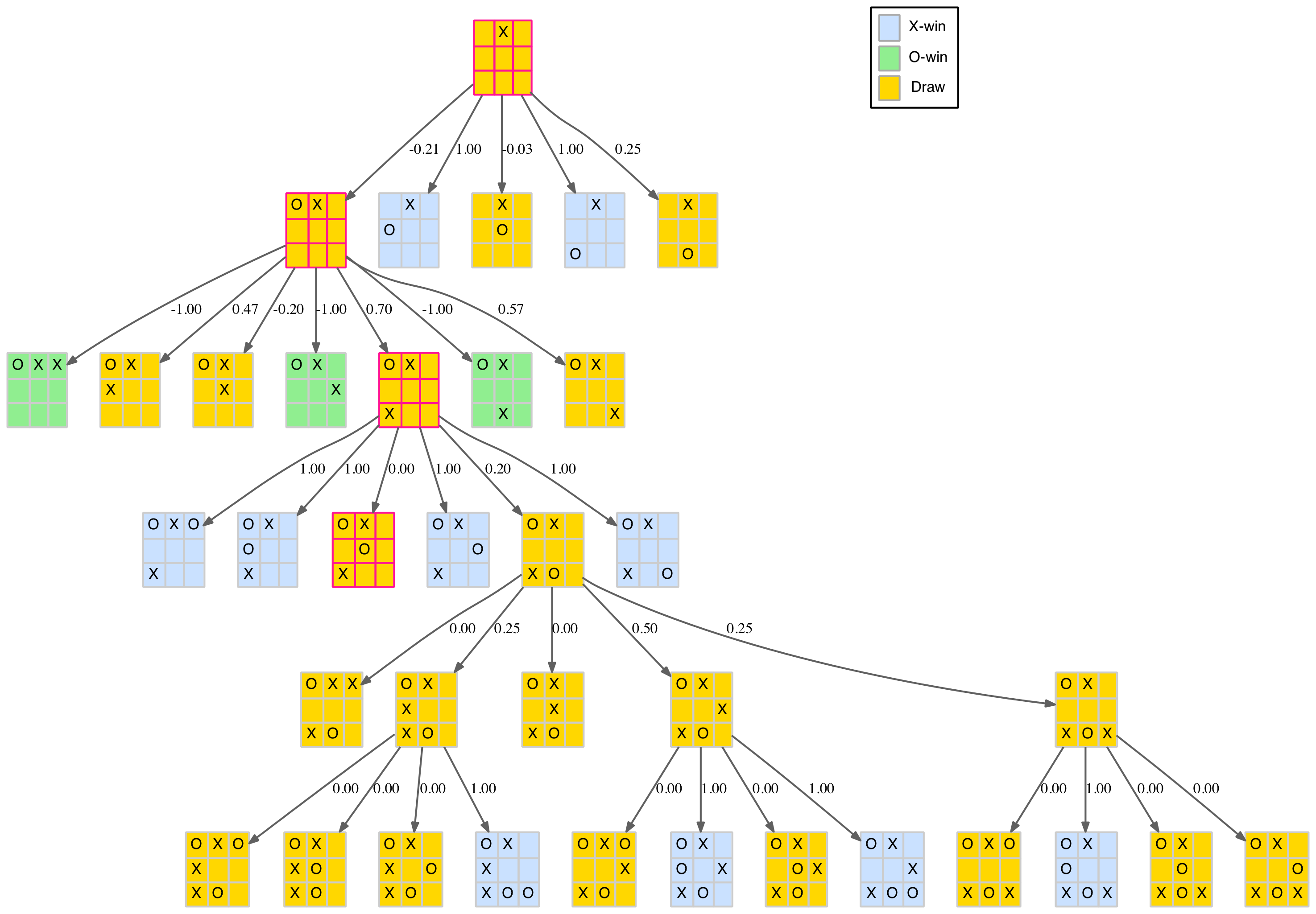
The full tree is still a bit large to comfortably display as one image but for the intrepid a link to the full tree in PDF format is provided at the end of this section, along with PDFs for each of the three first-move branches. The smallest of these branches, first move in the centre of the board, is shown below.


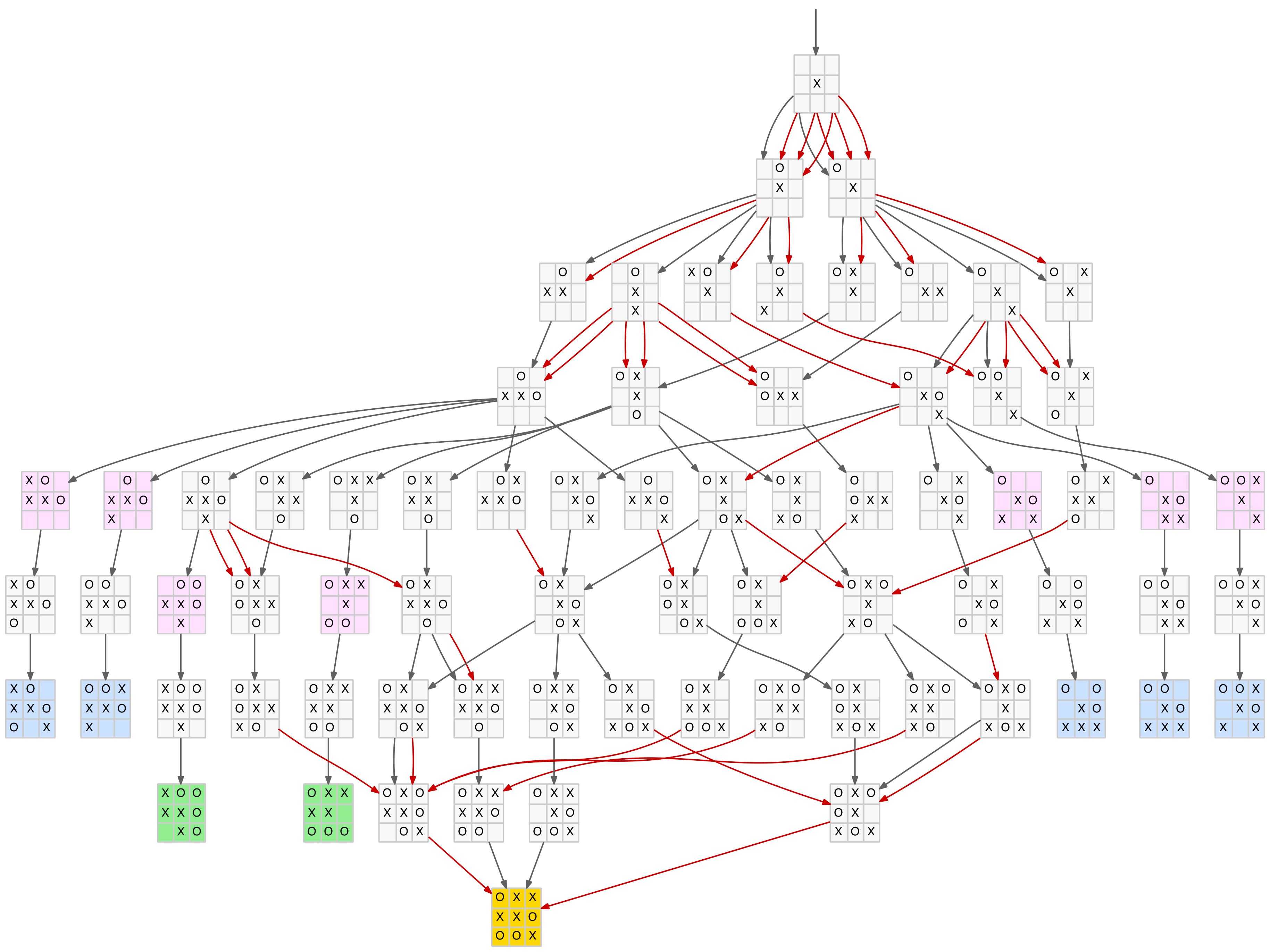
Branch of the full game tree

The nodes are colour-coded as follows:

  • Blue – X-win
  • Green – O-win
  • Gold – draw
  • Pink – fork

The dark edges (links between nodes) represent standard parent-child relationships. The red edges show the same parent-child relationships but with a symmetrical transformation included. That is, the child is derived from the parent with a new move added but then rotated or reflected to an existing node. Multiple red edges indicate that several of the parent’s child nodes transformed to the same final child node.

Note there is only one drawn board (the Island pattern – see above) as this pattern is the only one with an X-token in the centre square.

Links to the final game tree diagrams in PDF format:

The code that generates Graphviz for these diagrams is not included here but is relatively easy to derive from the tree walking code above as follows:

  • add a new atom to hold the dorothy data structure and pass it like ‘dups’ and ‘syms’
  • add a parent node argument that is passed down the recursion chain (for edge generation – see below)
  • add a dorothy node vector for each node to the dorothy data structure
  • add a dorothy edge vector connecting the node to its parent to the dorothy data structure
  • render the resulting dorothy data structure

Conclusion (Part 1)

We have shown that TTT can be represented as a 10-level game tree and that by accounting for duplicates, symmetries and forced moves, this tree can be reduced from over 500,000 nodes down to its essence of just 389 nodes. Despite always correctly blocking an opponents threats there are still won positions within this tree because of the existence of forked positions. These positions provide the main (only) tactical component of the game. Finally we learned that there are only three drawn position patterns.

In part 2 of this blog we will look at player strategies and seek to answer questions like:

  1. Can either player force a win?
  2. What is the best move in a given position?
  3. Can the game tree be reduced further?