Efficient Recursive Levenshtein (Edit) Distance Algorithm
Background
Levenshtein Distance is a way to ascribe a numeric distance between two sequences (often characters in a string or word) by counting the minimum number of insertion, deletion and substitution operations required to transform one sequence to the other.
As documented in Wikipedia (and elsewhere) there is an elegant recursive equation to determine the Levenshtein distance as follows:

If you think of transforming from sequence ‘a’ to sequence ‘b’ the first recursion represents a deletion from the ‘a’ sequence. The second recursion represents an insertion into the ‘b’ sequence, and the last recursion is either a substitution or a match (and skip over) depending on the equality check. The length is incremented in all cases except where there is a match.
When one sequence is exhausted (i.e. length=0) the length of the remaining sequence is added to the result (as either deletions or insertions depending which sequence is left).
Basic Computer Algorithm
The mathematical equation is fairly easily translated into a recursive computing function. The Clojure equivalent if translated literally would be something like:
(defn ld
  "Calculate the Levenshtein distance - basic literal code."
  [va vb i j]
  (cond
    (zero? (min i j)) (max i j)
    :else (let [k (if (= (va i) (vb j)) 0 1)]
            (min (+ (ld va vb (dec i) j) 1)
                 (+ (ld va vb i (dec j)) 1)
                 (+ (ld va vb (dec i) (dec j)) k)))))

(ld (vec " lawn") (vec " flaw") 4 4)  ; => 2
Literal translation of the Levenshtein equation
Note that each sequence is padded with an initial dummy character (blank in this case) to account for the difference between the one-based indexing used in the mathematical equation and the zero-based indexing used in computing. Without this adjustment the indexing gets messy and obscures the relationship with the equation.
A simpler and more idiomatic approach is to work directly with the sequences and avoid the indexing completely with code like this:
(defn ld
  "Calculate the Levenshtein distance - basic idiomatic code."
  [va vb]
  (cond
    (empty? va) (count vb)
    (empty? vb) (count va)
    :else (let [k (if (= (peek va) (peek vb)) 0 1)]
            (min (+ (ld (pop va) vb) 1)
                 (+ (ld va (pop vb)) 1)
                 (+ (ld (pop va) (pop vb)) k)))))

(ld (vec "lawn") (vec "flaw"))  ; => 2
Idiomatic (Clojure) representation of the Levenshtein equation
Both these implementations work and it’s not hard to find many examples of them on the Web (e.g. Rosetta Code) but they scale very poorly.
The solution tree grows by a factor of three for each level and the number of levels varies between the length of the shortest sequence and the sum of the lengths of both sequences. The function has a computing complexity of O(3n) which is essentially useless for anything but the shortest strings.
Some versions of this code employ ‘memorisation’ techniques in an attempt to improve performance. This helps because many nodes in the solution tree are duplicates which would otherwise be calculated over and over again. However memorisation introduces state and detracts for the functional purity of the solution. It also doesn’t address the underlying scaling problem.
Another approach is to use an iterative method based on a matrix representation. This is much more efficient (see below) but it masks the elegance of the original function.
Can we improve performance while maintaining the pure functional style of the equation? Two areas for improvement suggest themselves.
The first is the fact that as you recurse down the solution tree, the distance returned never reduces (i.e. it only gets larger or remains the same). So processing can stop once the result exceeds a previously calculated minimum.
The second is to note that two of the three recursion function calls use the third recursion result as input one recursion later. By passing this result down to the next recursive level, it doesn’t need to be recalculated.
We will look at these two optimisation methods below.
Upper Bound Optimisation
The idea is to pass an upper bound to the lower levels so that further processing can be avoided once that bound is reached. This is similar (but simpler) to alpha-beta pruning in two-person game trees. In this case, we need only a single alpha (or beta) value. It turns out that this approach provides significant pruning of the solution tree while vastly improves performance.
First let’s restructure the code above to pass a ‘running’ result down the tree. The new code looks like this:
(defn ld
  "Calculate the Levenshtein distance - basic with running result."
  [va vb res]
  (cond
    (empty? va) (+ res (count vb))
    (empty? vb) (+ res (count va))
    :else (let [k (if (= (peek va) (peek vb)) 0 1)]
            (min (ld (pop va) vb (+ res 1))
                 (ld va (pop vb) (+ res 1))
                 (ld (pop va) (pop vb) (+ res k))))))

(ld (vec "lawn") (vec "flaw") 0)  ; => 2
Idiomatic Levenshtein distance with a ‘running’ result
Here the initial call needs to pass the starting length of zero. This code doesn’t improve performance but it allows the result to be tested prior to further calls to lower levels.
Because the lower level calls can only ever increase (or keep the same) length, we can stop processing when the result equals (or exceeds) the current known minimum.
The following code introduces a fourth argument which holds the current known minimum. This value is updated after each branch is processed to let the next branch know the current best (minimum) value. Also the ‘substitution and match’ branch has been evaluated first because this is the only branch that can return a zero length increment which makes the ‘pruning’ minimum value more likely to be the lowest. This is equivalent to the heuristics applied is alpha-beta pruning where the player’s moves should be ordered with the likely strongest occurring first as this improves the pruning efficiency.
(defn ld
  "Calculate the Levenshtein distance - upper bound constraint."
  [va vb res minval]
  (cond
    (>= res minval) minval
    (empty? va) (+ res (count vb))
    (empty? vb) (+ res (count va))
    :else (let [k (if (= (peek va) (peek vb)) 0 1)
                r1 (ld (pop va) (pop vb) (+ res k) minval)
                r2 (ld va (pop vb) (+ res 1) (min r1 minval))
                r3 (ld (pop va) vb (+ res 1) (min r1 r2 minval))]
            (min r1 r2 r3))))

(ld (vec "lawn") (vec "flaw") 0 10000)  ; => 2
Levenshtein distance with an upper bound
The code introduces another termination case that tests whether the result (res) equals (or exceeds) the current best minimum (minval). If so, no further processing is performed as it will never improve on the current known minimum. Otherwise the next branch is evaluated with the lowest upper bound from the previous branches being passed on as the new upper bound.
Slightly more polished version
By taking advantage of Clojure’s multiple arity function definitions, we can simplify the call to the function by making the 2-arity function call the 4-arity version behind the scenes. This doesn’t change the functionality at all, it just hides some of the plumbing. The revised version is shown below.
(defn ld
  "Calculate the Levenshtein distance - upper bound constraint."
  ; ------ 2-arity
  ([seqa seqb]
   (let [minval (max (count seqa) (count seqb))]
     (ld (vec seqa) (vec seqb) 0 minval)))
  ; ------ 4-arity
  ([seqa seqb res minval]
   (cond
     (>= res minval) minval
     (empty? seqa) (+ res (count seqb))
     (empty? seqb) (+ res (count seqa))
     :else (let [k (if (= (peek seqa) (peek seqb)) 0 1)
                 r1 (ld (pop seqa) (pop seqb) (+ res k) minval)
                 r2 (ld seqa (pop seqb) (+ res 1) (min r1 minval))
                 r3 (ld (pop seqa) seqb (+ res 1) (min r1 r2 minval))]
             (min r1 r2 r3)))))

(ld "lawn" "flaw")  ; => 2
Upper bound Levenshtein distance
Note that we can set the minval initial value to the longest sequence as this is the worst case length (requiring every character to be replaced).
Performance Improvements
The table below shows the number of nodes processed by the original and bounded versions of the code for some sample sequences of increasing length. Indicative times are also provided but these are not rigorous benchmarks.
| Original | Bound | |||
|---|---|---|---|---|
| Sample Type | nodes/sample | msec/sample | nodes/sample | msec/sample |
| lawn->flaw | 1 | 0.10 | 13 | 0.01 |
| Mixed strings (len=5) | 841 | 0.49 | 32 | 0.01 |
| Mixed strings (len=6) | 4,494 | 2.51 | 64 | 0.02 |
| Mixed strings (len=7) | 24,319 | 13.48 | 134 | 0.03 |
| Mixeds strings (len=8) | 132,864 | 73.08 | 254 | 0.06 |
| abcdefghi->123456789 | 731,281 | 448.00 | 9841 | 2.35 |
| a12345678->123456789 | 731,281 | 418.00 | 74 | 0.02 |
| levenshtein->einstein | 1,242,912 | 763.00 | 264 | 0.07 |
| levenshtein->meilenstein | 22,523,360 | 12,992.00 | 365 | 0.10 |
It is clear that the bounded version is a substantial improvement over the original version. This is most obvious as the length of the strings increase. However, the bounded version itself can fluctuate significantly depending on the input values as seen by the two highlighted lines in the table above. Here the input strings are the same length but the nodes processed vary by a factor of over 100.
Reuse of the ‘substitution’ value
The second optimisation approach is revealed by considering the following diagram showing two levels of recursion for the original Levenshtein equation.

The (i-1,j-1) term, also known at the substitution term, in the first recursion is also used by the other two terms at the next level down. So some additional optimisation can be achieved by preserving this value and passing it down to the next level. As only four new terms are calculated, instead of six, there should be a modest but noticeable improvement.
The modified code adds two new parameters that represent the ‘left’ (i-1,j) and ‘right’ (i,j-1) substitution value previously calculated. The code starts to get a little more opaque but the main theme is still relatively clear.
(defn ld
  "Calculate the Levenshtein distance - upper bound constraint
  and reuse of the 'substitute' term value."
  ([seqa seqb]
   (let [minval (max (count seqa) (count seqb))]
     (ld (vec seqa) (vec seqb) 0 minval nil nil)))
  ;
  ([va vb res minval r2 r3]
  (cond
    (>= res minval) minval
    (empty? va) (+ res (count vb))
    (empty? vb) (+ res (count va))
    :else
    (let [k (if (= (peek va) (peek vb)) 0 1)
          r1 (ld (pop va) (pop vb) (+ res k) minval nil nil)
          r2 (if r2 r2 (ld (pop va) vb (+ res 1) (min r1 minval) nil r1))
          r3 (if r3 r3 (ld va (pop vb) (+ res 1) (min r1 r2 minval) r1 nil))]
      (min r1 r2 r3)))))

(ld "lawn" "flaw")  ; => 2
Performance
The table below compares the bounded, and the bounded and reuse versions.
| Bound | Bound and reuse | |||
|---|---|---|---|---|
| Sample Type | nodes/sample | msec/sample | nodes/sample | msec/sample |
| lawn->flaw | 13 | 0.01 | 13 | 0.01 |
| Mixed strings (len=5) | 32 | 0.02 | 24 | 0.01 |
| Mixed strings (len=6) | 64 | 0.02 | 42 | 0.01 |
| Mixed strings (len=7) | 134 | 0.05 | 76 | 0.03 |
| Mixed strings (len=8) | 254 | 0.10 | 126 | 0.04 |
| 123456789->abcdefghi | 9,841 | 3.15 | 2377 | 0.78 |
| 123456789->a12345678 | 53 | 0.02 | 53 | 0.02 |
| levenshtein->einstein | 264 | 0.11 | 136 | 0.05 |
| levenshtein->meilenstein | 365 | 0.13 | 205 | 0.06 |
There is a small additional improvement by reusing the ‘substitution’ value. This is most noticeable where the bounded version works less well (highlighted rows).
Conclusion
The ‘standard’ recursive function to compute the Levenshtein distance is elegant but scales very badly, O(3n), which makes it impractical (and dangerous) for most applications. By adding an upper-bound constraint the recursive function can be substantially improved. Some further improvement is achieved by reusing the ‘substitution’ value. These improvements arise by significantly reducing the number of nodes in the solution tree that need to be processed.
Iterative version
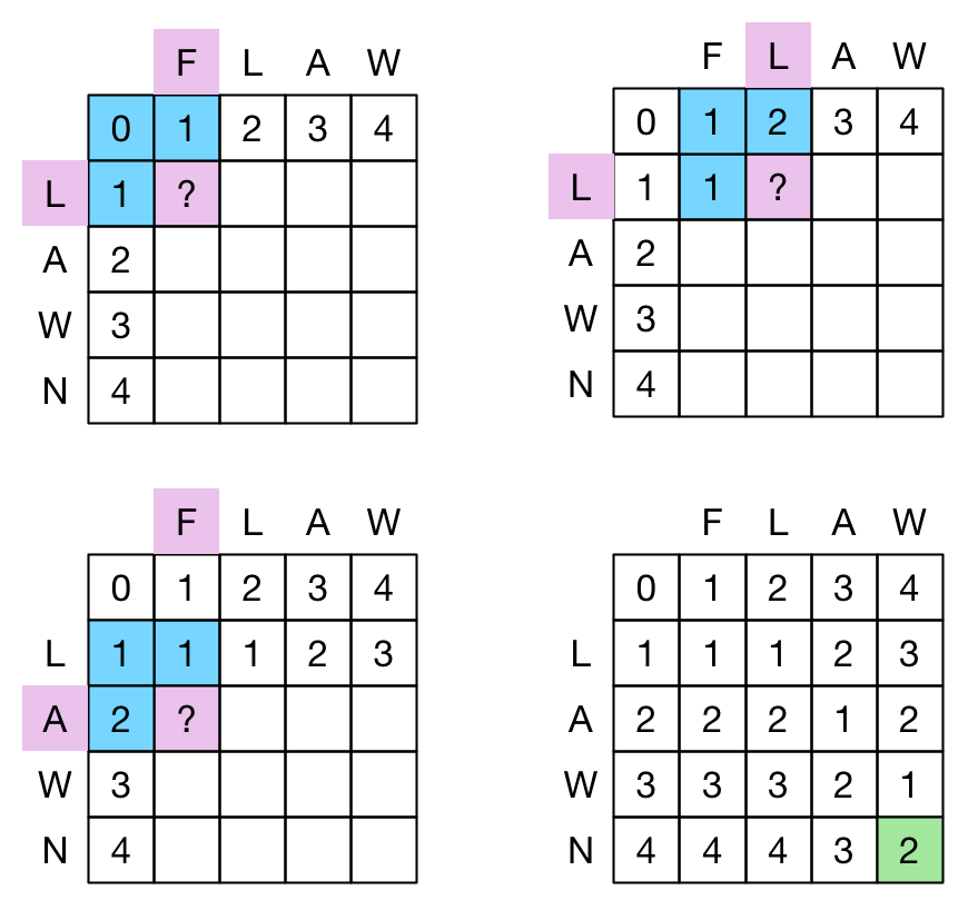
Levenshtein distance can be represented in a matrix or grid format. One sequence is laid out at the top, horizontally, and the other is laid out to the left, vertically. Each is prepended with a notional ‘null’ entry and the initial distance (0, 1, 2, …) from this null entry is entered in the first row and first column of the grid.
From this starting position the grid is filled in cell by cell, left to right, top to bottom. The cell values represent the Levenshtein distance between the two sub-sequences – one from the left to the current cell’s horizontal location and the other from the top to the current cells vertical location. The ‘rule’ for determining the value of the next cell is to take the minimum of:
- The cell immediately above it plus one
- The cell immediately left of it plus one
- The cell immediate above and left of it plus one if the corresponding sequence entries are different, or zero if they are the same
When the grid is completed, the bottom right value is the Levenshtein distance between the two sequences. An example is shown in the following diagram (“?” shows the cell to be determined, blue cells are the ones used as input, along with the highlighted sequence entries which are tested for equality).
There are clearly strong parallels here between the recursive equation and the grid construction.
The big difference between the methods is that the grid construction is at worst O(n2). The grid method also lends itself to an iterative implementation. A simple Clojure iterative version is shown below. It uses two row variables rx and ry that progressively move down the grid. The ry row is built up from the rx row above it, and, its own last lefthand value. Once completed, the rx row is replaced with the ry row and the process is repeated.
(defn ld-grid-iter
  "Calculate the Levenshtein (edit) distance iteratively using
  a grid representation"
  [seqa seqb]
  (let [va (vec seqa)
        vb (vec seqb)
        clen (inc (count va))
        rlen (inc (count vb))
        rx (vec (range clen))]
    (loop [r 1, c 1, rx rx, ry (assoc rx 0 1)]
      (if (= r rlen)
        (peek rx)
        (if (= c clen)
          (recur (inc r) 1 ry (assoc ry 0 (inc r)))
          (let [k (if (= (va (dec c)) (vb (dec r))) 0 1)
                ry (assoc ry c (min (+ (rx c) 1)             ; above
                                    (+ (ry (dec c)) 1)       ; left
                                    (+ (rx (dec c)) k)))]    ; diagonal
            (recur r (inc c) rx ry)))))))

(ld-grid-iter "lawn" "flaw")  ; => 2
Iterative grid version of Levenshtein distance
The performance comparison of the ‘bounded and reuse’ recursive version developed above and the iterative grid version for the same sample set is shown in the following table.
| Bound and reuse | Iterative grid | |||
|---|---|---|---|---|
| Sample Type | nodes/sample | msec/sample | nodes/sample | msec/sample |
| lawn->flaw | 13 | 0.01 | 16 | 0.01 |
| Mixed strings (len=5) | 24 | 0.01 | 25 | 0.01 |
| Mixed strings (len=6) | 42 | 0.02 | 36 | 0.01 |
| Mixed strings (len=7) | 76 | 0.02 | 49 | 0.01 |
| Mixed strings (len=8) | 126 | 0.04 | 64 | 0.01 |
| 123456789->abcdefghi | 2,377 | 0.75 | 81 | 0.01 |
| 123456789->a12345678 | 53 | 0.01 | 81 | 0.02 |
| levenshtein->einstein | 136 | 0.11 | 88 | 0.03 |
| levenshtein->meilenstein | 205 | 0.08 | 121 | 0.03 |
In general, the iterative grid version outperforms the recursive version, as you would expect, but the recursive version holds up surprising well at least for typical word-length sequences (less than around a length of 12).
There is scope to optimise the iterative version using upper bounds in a similar way to the recursive version although this is not explored here. And of course it is possible to turn the iterative grid version into a recursive grid version for the functional purist with code like:
(defn ld-grid-recursive
  "Calculate the Levenshtein (edit) distance recursively using
  a grid representation"
  ([seqa seqb]
   (ld-iter-recursive seqa seqb 1 (vec (range (inc (count seqa))))))
  ;
  ([seqa seqb r vx]
  (if (empty? seqb)
    (peek vx)
    (let [r-fn (fn [v [a x0 x1]]
                 (let [k (if (= a (first seqb)) 0 1)]
                   (conj v (min (+ x1 1)           ; above
                                (+ (peek v) 1)     ; left
                                (+ x0 k)))))       ; diag
          vx (reduce r-fn [r] (map vector seqa vx (rest vx)))]
      (ld-grid-recursive seqa (rest seqb) (inc r) vx)))))

(ld-grid-recursive "lawn" "flaw")  ; => 2
Recursive grid version of Levenshtein distance